Results of the Steady-State Calculation
Evaluate the results of the steady-state calculation: false color in the network, result tables, pressure profile to the index point and pump design
Overview
After the calculation, VICUS Districts presents the results per operating point: as false color in the 3D network, in result tables for pipes, energy plants and consumers, as a path profile along a supply path (pressure profile to the index point) and in the pump design. The results are part of the project file and remain available after reopening the project.
Access
 Steady-State Calculation button in the left-hand toolbar. At the top, the view contains the network selection and the operating-point list, and below it the three areas Results, Path Profile and Pump Design.
Selecting an Operating Point
The Operating Point table lists all calculated operating points with their status. Selecting a row switches all displays (colors, tables, profile, pump design) to that operating point.
| Status | Meaning |
|---|---|
| Valid | Calculation converged, no anomalies |
| Warning | e.g. non-converged nodes, very low temperatures or deviation from the target temperature / pressure difference at the index point; a detail button opens a dialog with recommended solutions |
After changes to the network or to referenced database elements, the note “Network has been changed - results may be outdated” appears — then repeat the calculation.
Results Area
The Results area contains four tabs: Pipe Network, Energy Plants, Consumers and Summary. The selected result quantity colors the network in the 3D scene (false color with color legend) and highlights the corresponding table column.
| Element | Function |
|---|---|
| Result quantity | Quantity for network coloring and column highlighting |
| Adjust table | Show and hide table columns |
| Show flow direction | Arrowheads on the pipes indicate the calculated mass-flux direction (default: enabled) |
| Consider geometric height | includes the geodetic pressure component from the node heights in the pressure quantities (default: enabled) |
| Edit legend … | Adjust the value range (minimum/maximum) of the color scale |
 Copy Copy | Copy the table to the clipboard |
Each table row also contains a Select in scene button that selects the respective object in the 3D view.
Consider geometric height is enabled by default and affects the display only: both variants are stored in the results, so switching does not require a recalculation. Switch the option off and the displayed pressures lack exactly the component that governs whether the operating pressure limits are met — for judging the highest and lowest pressure, leave it on. If all nodes still sit at z = 0, for instance because no elevation query has been run yet, the option has no effect.
Pipe Network
Use the Supply / Return options to select the displayed network side. Available result quantities:
Pressure [bar], Pressure loss per meter [Pa/m], Temperature [°C], Power [kW], Utilization [%], Relative reserve [%], Reserve capacity [kW], Maximum capacity [kW], Volume flow [m³/h], Mass flux [kg/s], Velocity [m/s], Pressure difference [mbar], Pressure exceedance [bar], Heat loss [W], Heat loss per meter [W/m].
Utilization, reserve and capacity refer to the maximum pipe pressure loss configured in the calculation dialog.
Pressure exceedance [bar] reports, per pipe, the amount by which the operating pressure exceeds the nominal pressure rating PN of the assigned pipe type; as long as the limit holds, the value is 0. The value is always ≥ 0 — a shortfall is not reported here. Gauge is checked against gauge, so the comparison is exact; a pipe with no nominal pressure rating assigned is not checked.
The quantity looks at the upper limit only, and at pipes only — valves, fittings and plant components with a rating of their own are left out. The evaporation check against the minimum operating pressure is not part of it; it sits in the status line of the path profile and in the network report. The limits themselves are described in Meeting operating pressure limits in heat networks.
Good to know
Utilization [%] and Relative reserve [%] are your quickest view of the sizing quality: routes near 100 % utilization are bottlenecks, routes with high reserve are oversized. Since both quantities refer to the configured maximum pipe pressure loss, you always assess the same reference value as in the pipe sizing. Color the network by them via the result quantity to spot reserves and bottlenecks at a glance.
Energy Plants and Consumers
Tree view per network node with the elements of the assigned plant. Result quantities include: pressure difference [bar], temperature difference [K], supplied heat [kW] (energy plants) or extracted heat [kW] (consumers), inlet and outlet temperature [°C], volume flow [m³/h], inlet and outlet pressure [bar]; depending on the plant type additionally heating power [kW], COP [-], pump efficiency [%] and connection-load utilization [%].
Summary
Key figures of the operating point as a table (name, value, unit):
- Index point: governing consumer with total pressure difference, pressure difference of the pump(s) and temperature difference. With a central pump, the index point is the consumer with the smallest pressure difference; with decentralized pumps, the consumer with the highest.
- Energy plants: supplied or dissipated heat per plant, where applicable COP and pump pressure difference, as well as sum values over all plants.
- Height differences: highest point of the network and the position of the energy plants relative to it. This row is the way into the pressure assessment: the minimum pressure becomes governing at the highest point of the network, the maximum pressure at the lowest — roughly 10 m of height difference correspond to 1 bar. Which limits have to be met is described in Meeting operating pressure limits in heat networks.
- Pipe network: heat-loss power (total, per length and relative to the injected heat), where applicable heat gains, as well as the share of the fittings in the total pipe pressure loss.
Path Profile (Pressure Profile)
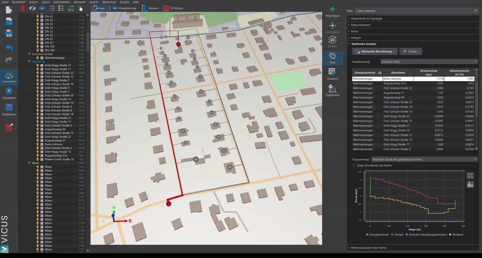
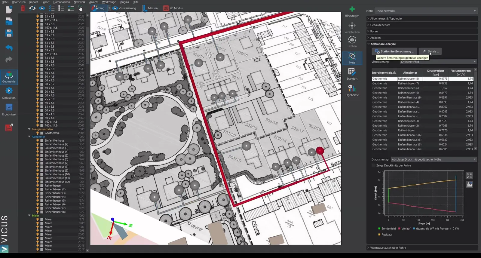
The Path Profile area shows the course of a result quantity along the supply path from an energy plant to a consumer — from the outlet of the source plant via the supply and the consumer plant back through the return. A typical application is the pressure profile to the index point as a basis for the pump design.
- Select Energy plant and Consumer from a list, by clicking in the 3D scene (pick mode), or zoom to the selected object.
- Quantity: Temperature [°C], Pressure [bar] or Height [m] (geodetic height profile of the path).
- Consider geometric height adds the component to the displayed pressure course; when disabled, only friction losses are shown.
Checking the Pressure Limits
Below the selection fields sits a status line that checks the pressure course of the selected path against two limits. What is checked is always the operating pressure, that is the gauge pressure including the geodetic component — regardless of which quantity the chart currently shows, because the limits apply to the pressure that actually stands in the pipes.
| Checked quantity | Limit |
|---|---|
| Highest operating pressure | ≤ lowest nominal pressure rating PN of the pipes on the path; gauge against gauge, so the check is exact |
| Lowest operating pressure | ≥ min. operating pressure: vapour pressure at the hottest point of the path plus the Minimum pressure margin from the general settings, less the ambient pressure |
The line opens with All pressure limits are complied with. or Not all pressure limits are complied with. and follows it with one sentence per limit, naming the value reached, the limit and — where a limit is missed — the deviation (exceeded by or undercut by). If a limit cannot be determined, for instance because the pipes of the path carry no nominal pressure rating or the operating point supplies no fluid temperatures, the corresponding sentence is omitted; if neither can be determined, the line stays empty.
The network report documents the same check as a table with a colored swatch — and states there in addition how the limits are formed. The technical reasoning behind the margins is covered in Meeting operating pressure limits in heat networks.
The Chart tab plots the curves for source plant, supply, consumer plant and return over the route length. The Table tab lists each segment of the path individually — pipes as well as fittings — with the columns node id, plant/pipe, component, temperature [°C], pressure loss dp [mbar], p_in and p_out [bar], mass flux [kg/s], volume flow [m³/h], length l [m], dp/l [Pa/m], velocity v [m/s], zeta value [-] and height [m]. Use  Export table as CSV to save the listing as a file, and Copy to transfer it to the clipboard.
The profile quantity Height [m] and the table column Height [m] are the tools for checking the node heights numerically: the chart shows the height course of the path, the table the value per segment, and the CSV export lets you go through it row by row — this is how you find nodes that were inadvertently left at 0. The values are node heights relative to the project origin, not absolute terrain elevations above sea level; for the pressure assessment only the difference counts.
Pump Design
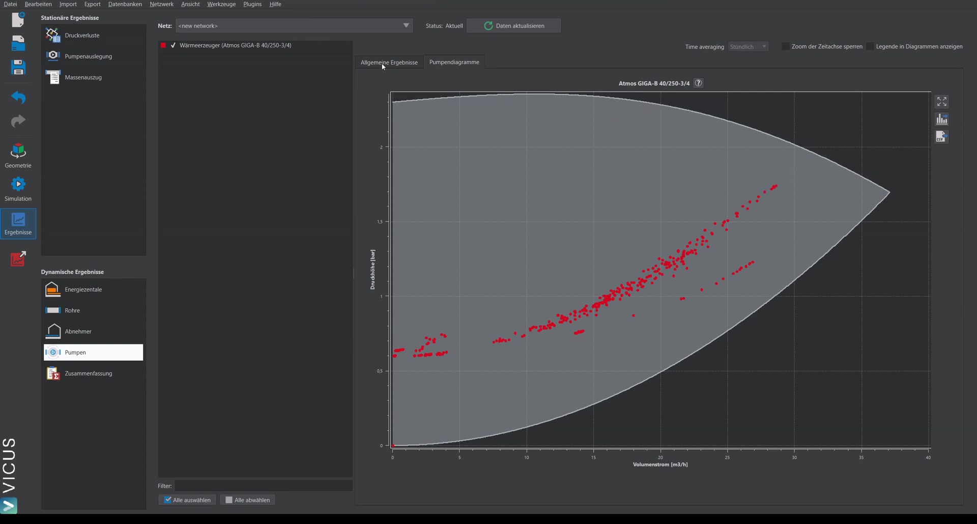
The Pump Design area lists the pumps of the selected operating point with their operating point (volume flow, pressure difference). For the selected pump, VICUS Districts suggests suitable pumps from the database:
| Element | Function |
|---|---|
| Assign | assign the selected database pump to the plant |
| Edit plant … | opens the editor of the associated plant |
| Custom characteristic curve … | create your own pump characteristic curve |
| Remove characteristic curve | reset the pump characteristic curve to default values |
| Number of parallel pumps | parallel pumps split the volume flow evenly at equal head; the total characteristic curve is stretched horizontally by the factor N |
The chart shows the pressure difference [bar] over the volume flow [m³/h] with the pump characteristic curve, plant characteristic curve and operating point. After assigning a pump, the note “Pump has been reassigned - recalculation recommended” appears — run the steady-state calculation again so that the operating point matches the new characteristic curve. Plants with a simplified model cannot receive a pump characteristic curve; switch to a detailed model in the plant editor for that.
Saving and Export
- The results are saved in the project file (including undo/redo) and restored on reopening. A checksum detects intervening changes to the network or databases and marks the results as outdated.
- For plans, export the result display as DXF; the network itself can additionally be exported as GIS data. All result tables can be copied to the clipboard; the table of the path profile can additionally be exported as CSV.
- The network report collects the key figures, pressure profiles, pipe utilization and pump design of the selected operating points into one continuous document (PDF, Word, HTML or AsciiDoc). The check against the nominal pressure rating and the minimum operating pressure is carried out there.