Steady-state calculation & checking the sizing

Overview

In this second part, the network is calculated hydraulically and the pipe sizing is checked. The goal is to ensure that the pressure losses in the network can be handled by the available pumps.

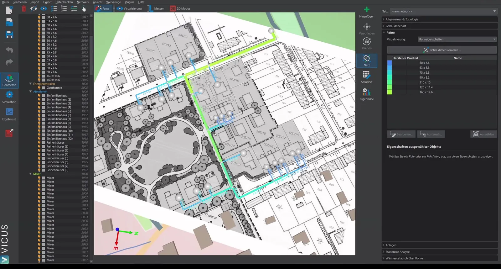
Adjusting the display

Under Visualization, various display options can be set:

• Show the pipe network smaller so it is easier to recognize.
• Set a uniform text color.
• Adjust the text scaling.

Setting up the plants

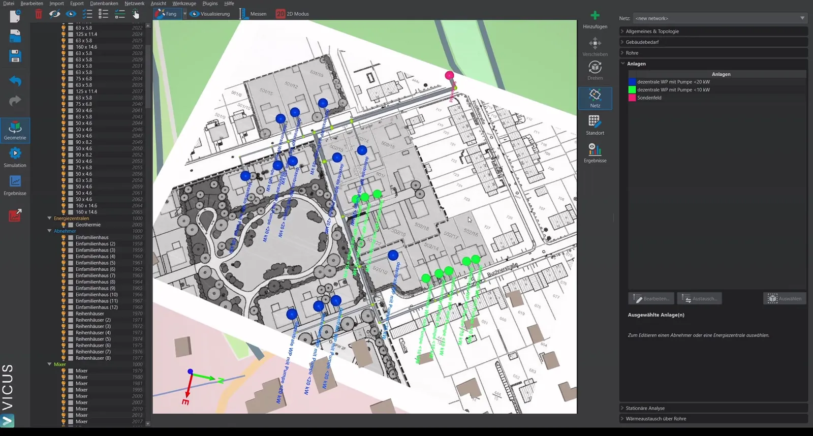
On the Plants tab, decentralized heat pumps are already assigned. A new plant must be created for the energy plant (borehole field):

1. Select the energy plant and click Assign new plant.
2. Create a new plant in the database.
3. Select the geothermal borehole field as the element.
4. Add a quadratic pressure-loss element for the distributor as a second element (e.g. 0.1 bar at 45 m³/h volume flow).
5. Connect the elements in series.
6. Assign meaningful names (e.g. “Distributor” for the pressure-loss element, “Borehole field” for the plant).

Parameterizing the geothermal borehole field

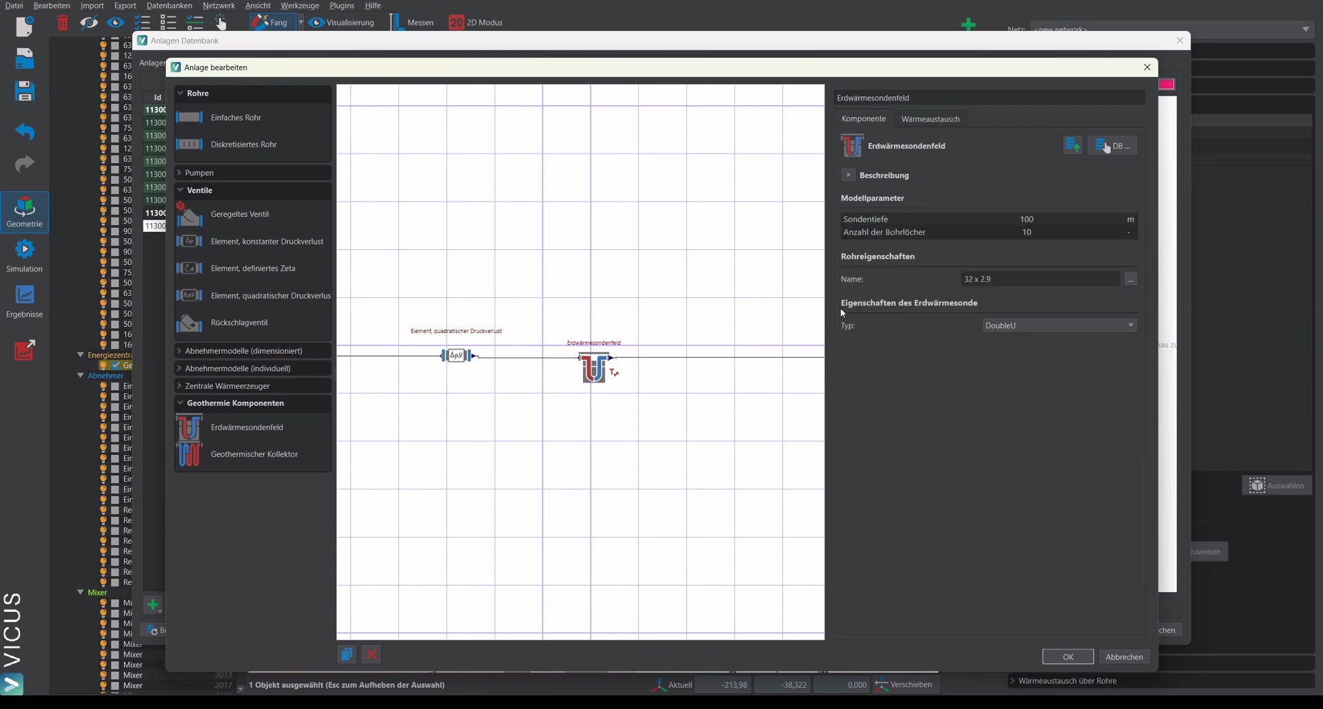
For the borehole field, the hydraulic consideration is performed first. The borehole sizing is done in a separate step. In this example, 25 boreholes are configured, each 100 m deep with 32 mm pipe.

Performing the steady-state calculation

1. Open the steady-state calculation dialog.
2. The supply temperature is specified for the fluid viscosity.
3. Set the temperature difference to 3 Kelvin.
4. Choose decentralized pumps as the supply.
5. Start the calculation.

Evaluating the results

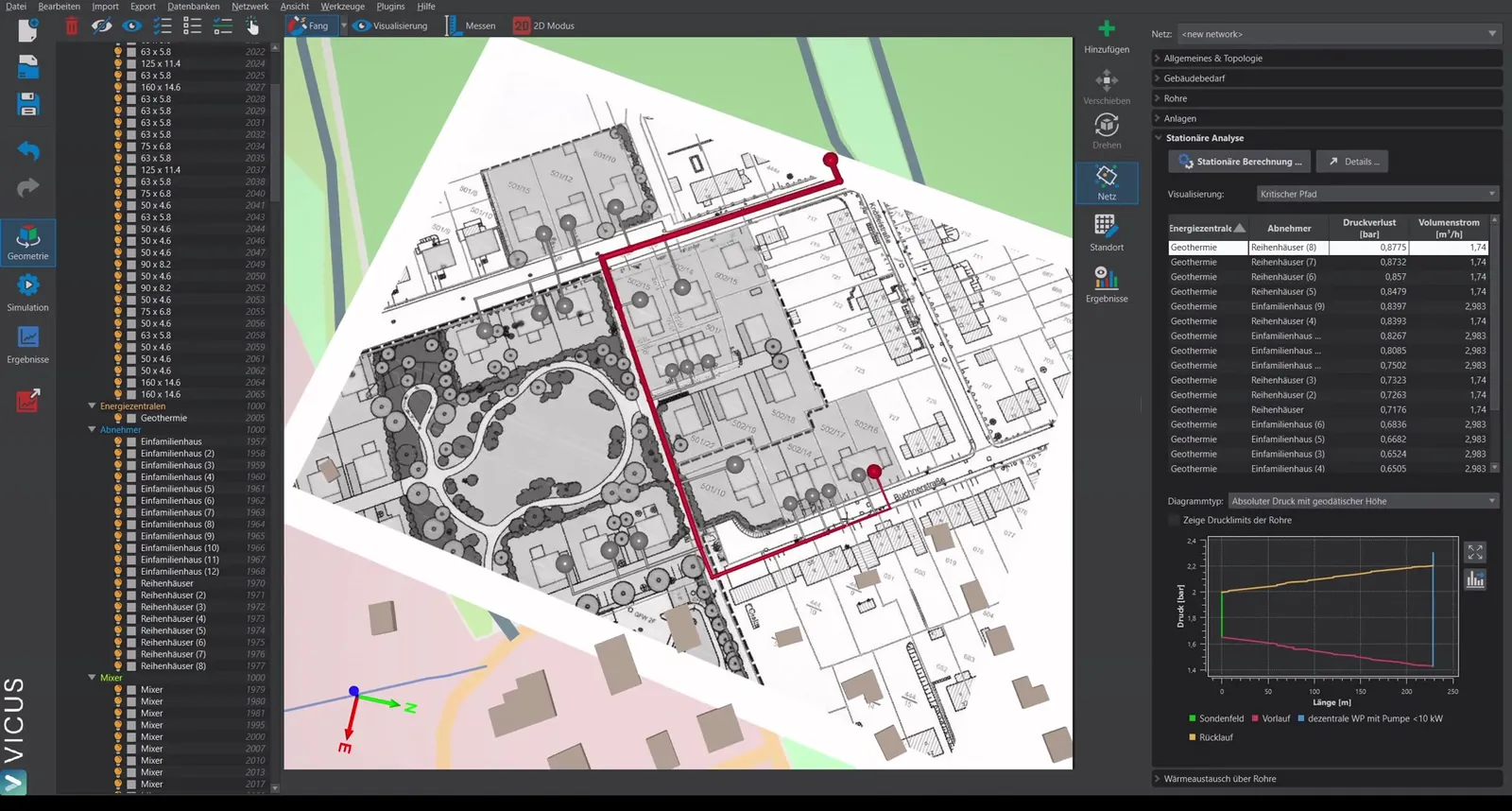
After the calculation, the following are displayed:

• Pressure loss at the worst point (e.g. 0.87 bar)
• Visualization of various calculation results
• Via the Details button: a detailed breakdown of the pressure loss (distributor, borehole field, network) along with the associated volume flow

Checking the pump sizing

The pump sizing shows whether the stored pumps can handle the calculated pressure loss. In a cold district heating network with decentralized pumps, these are usually already built into the heat pump.

If the pressure loss exceeds the pump capacity, the sizing must be adjusted.

Optimizing the sizing

To reduce the pressure loss, the sizing method can be changed:

1. Open the pipe sizing dialog.
2. Switch from maximum pressure loss per pipe length to maximum pump head.
3. Select all entries with Shift-click and enter the maximum head (e.g. 0.75 bar).
4. Perform the sizing again.

Checking the result

After a renewed steady-state calculation, the maximum pressure loss should be within the specified value (e.g. 0.7 bar for a specification of 0.75 bar). The pump sizing now shows that the operating point lies within the pump’s operating range.

Assigning pumps

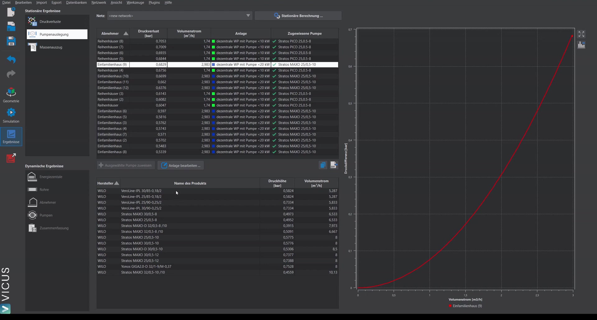
If no pump has been assigned to a plant yet, you can select an entry in the pump sizing and assign the pump to the plant. It is then automatically assigned to all identical plants as well.

The project is now fully prepared to be simulated in the next step.

Video tutorial