Introduction to VICUS Districts

First steps

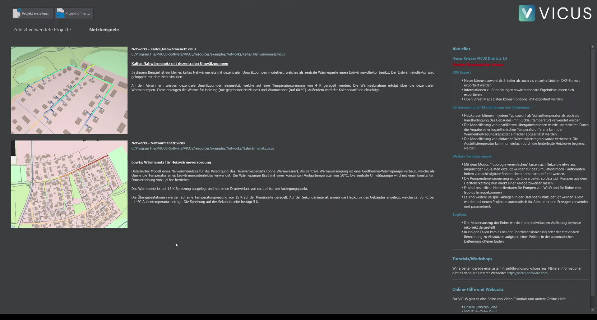
When starting VICUS Districts for the first time, it is advisable to explore the integrated examples. To do so, switch to the Network examples tab and open an example project. This lets you quickly understand how a network is built, how a steady-state calculation is performed and how simulation results are evaluated.

User interface

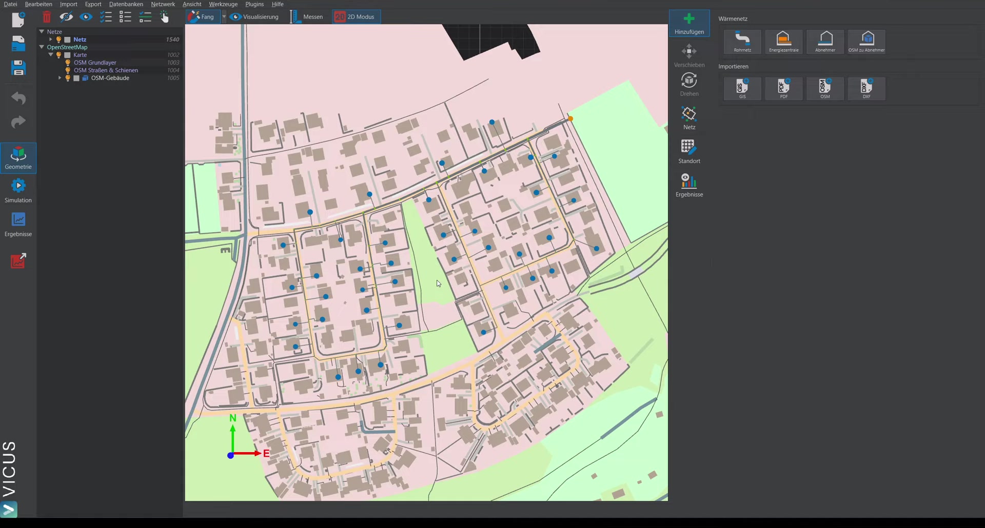
Navigation tree (left side)

The navigation tree on the left side manages all project elements:

• Selecting elements: Click an element in the tree to highlight it in the map view. Conversely, clicking a network element in the map activates the corresponding element in the tree.
• Controlling visibility: Via the light-bulb icons, layers or individual elements can be shown and hidden.
• Renaming: By double-clicking an element in the tree, you can rename it.

Interaction and control

• Additive selection: When selecting multiple elements, these are added to the selection.
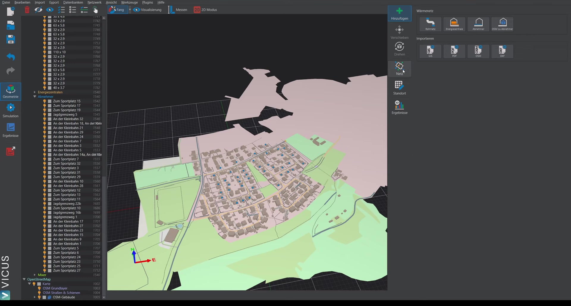
• Deselecting: With ESC, the entire selection is cleared.
• 2D/3D view: Via the button at the top, you can switch between 2D and 3D mode. In 3D mode, you navigate with the left mouse button.
• Navigating faster: Hold down the spacebar to increase the movement speed – particularly useful with large models.

Adding elements (right side)

On the right side, you can create new elements:

• Draw the network and add pipe elements
• Position consumers and energy plants
• Import data (GIS, PDF, OpenStreetMap, DXF)

Network planning and configuration

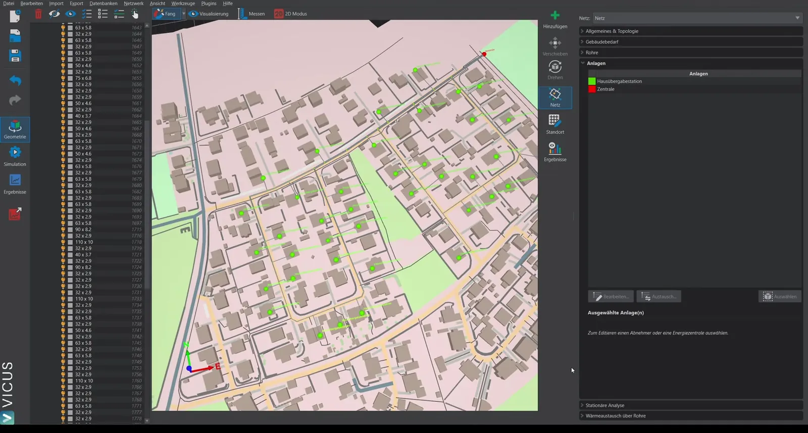
When you activate the Network element on the left side, various configuration tabs become available on the right side:

General tab

Here you define the fluid and use topology tools:

• Connect consumers automatically
• Set elevations automatically
• Simplify the network topology

Building demand tab

Visualization of the connection loads in the network. Depending on the mode set, the heating energy demand and further properties can also be displayed.

Pipe sizing tab

Shows the assigned pipe dimensions directly in the scene. When selecting a pipe, you get detailed information on the pipe kind, pipe type and length. Individual network sections can be locked for pipe sizing.

Visualization options: Via the visualization button at the top, you can adjust the display:

• Scale consumer nodes and pipes larger/smaller
• Show/hide labels (with very large models, the text display can slow down the rendering)
• Change the font size and text color

Plants tab

Definition of the plant components:

• House transfer stations (simple or detailed)
• Energy plants (several within the network are also possible)

Ground conditions tab

Setting of the ground boundary conditions for the network, e.g. ground temperatures and boundary conditions for the heat-loss calculation.

Calculation and simulation

Steady-state calculation

The steady-state calculation provides a snapshot of the network performance:

• Display of the pressure curve
• Identification of the worst point (hydraulically most unfavorable consumer)
• Overview of all consumers with pressure loss and volume flow
• Detailed listing of the branch with all installed parts and their respective pressure losses
• Pump sizing: Automatic suggestion of suitable pumps from the integrated database

Dynamic simulation

Under the Simulation section you find:

• Climate data: Import of weather data directly from the German Weather Service (DWD) or loading your own climate data
• Simulation settings: Adjustment of the parameters for the dynamic simulation
• Hourly results: After the simulation you obtain hourly-resolved evaluations of heating power, COP, heat losses of the pipe network and further key figures

Reports and outputs

• Bill of materials: Complete listing of all pipes as well as all pipe fittings (elbows, T-pieces, reducers, etc.)
• Result summary: Overview of the most important simulation key figures

Video tutorial