Building demand in the detail editor
The Edit building demand dialog for a single consumer: building type, Heating, Domestic hot water and Cooling tabs, preview chart and value table
Overview
The Edit building demand dialog is the detail editor for the demand of a single consumer that derives its demand model from predefined time series. It combines heating, domestic hot water and cooling demand in three tabs, shows the generated demand profile as a chart and value table, and applies the values to all selected consumers. The tabular editing of all consumers, by contrast, is described in Editing building demands.
How to open
The dialog is opened from the Building demand tab of the network properties when the consumer uses the Predefined time series demand model:
 Edit demand parameters … with exactly one selected consumer
- Edit all demand parameters … with several selected consumers
For a multiple selection, the dialog is populated with the values of the first selected consumer and, on applying, overwrites all selected consumers with the same values. The Applies to n consumers field at the bottom shows the number of affected consumers.
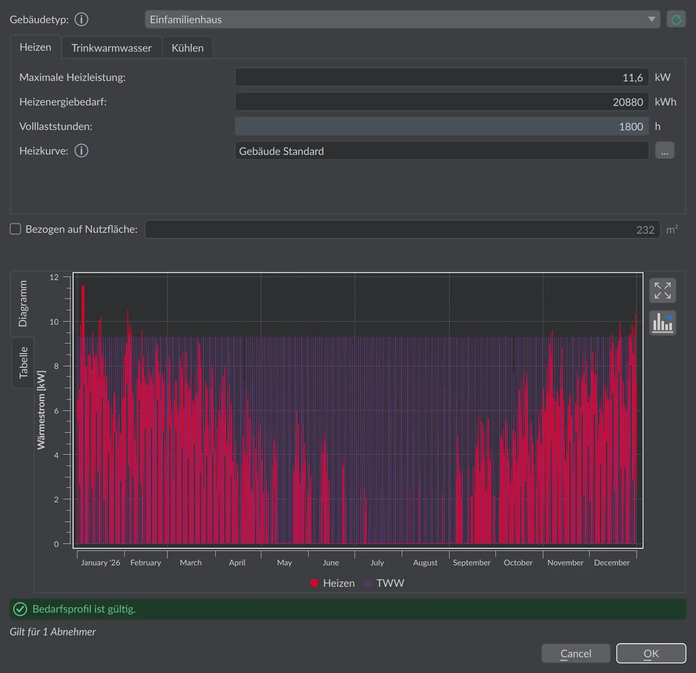
Building type and default values
Above the tabs are the building type and the default values button:
| Element | Meaning |
|---|---|
| Building type: | Selects the typical demand profile (single-family house, office building, school, etc.), which determines the shape and characteristic values of the annual profiles for heating, cooling and domestic hot water. The available types are listed under Editing building demands |
 Set default values Set default values | Resets all values (usable area, powers, energies, domestic hot water) to the default values of the current building type, after a confirmation prompt |
If a different building type is chosen, the Change building type dialog opens. Since the profile shape changes, it is possible to decide there how to handle the existing values:
| Option | Behavior |
|---|---|
| Use default values for this building type | Fully applies the default values of the new type |
| Keep maximum heating power and use adjusted default values for this building type | Keeps the peak power, calculates the annual energy from the new profile shape (default) |
| Keep energy demand and use adjusted default values for this building type | Keeps the annual energy demand and adjusts the remaining values |
| Only change building type and keep all properties | Changes only the type, keeps all entered values |
If the dialog is canceled, the previous building type is retained.
Heating tab
| Field | Unit | Editing |
|---|---|---|
| Maximum heating power: | kW | Input |
| Heating energy demand: | kWh | Input |
| Full-load hours: | h | calculated (heating energy demand / max. heating power) |
| Heating curve: | – | Selection via … (Choose heating curve from database); shows None, the curve name or Invalid heating curve |
If the maximum heating power is changed, the heating energy demand scales in the same ratio, so that the full-load hours remain constant. The heating curve defines how the secondary-side supply temperature changes with the outdoor temperature; the same curve can be reused across multiple consumers.
Domestic hot water tab
| Element | Unit | Editing |
|---|---|---|
| Use domestic hot water (DHW) | – | Check box (default: active). When disabled, it locks all DHW fields |
| DHW preparation mode: | – | In scheduled time windows (default) or In addition to heating |
| Ratio DHW/heating power: | – | Input, default 0.80, range 0.01 – 10.0. Only visible in In scheduled time windows mode |
| DHW supply temperature: | °C | Input, default 50, range 20 – 100. Only visible in In scheduled time windows mode |
| DHW energy demand: | kWh | Input |
| DHW share: | % | calculated (share of the DHW energy in the total heat demand) |
The two preparation modes determine how the DHW profile is combined with the heating profile:
| Mode | Behavior |
|---|---|
| In scheduled time windows | Storage model: DHW is generated in two preparation windows per day (02:00 – 04:00 and, as overflow, 12:00 – 14:00) at the DHW peak power. During these windows the heating is suspended and its energy is distributed over the remaining hours; preparation is done at the set DHW supply temperature. The DHW peak power results from ratio × max. heating power |
| In addition to heating | Simple model: the scaled DHW profile is added to the heating profile, without preparation windows and without a separate DHW supply temperature. The Ratio DHW/heating power and DHW supply temperature fields are omitted |
In practice
The two preparation modes lead to noticeably different peak loads. In scheduled time windows bundles the DHW preparation into charging windows and suspends the heating in return - this models a DHW storage tank and limits the simultaneous peak. In addition to heating, by contrast, adds DHW undamped onto the heating load and thus produces the more conservative, higher connection load. Choose the mode according to whether a storage tank absorbs the DHW peak in the real building.
Cooling tab
| Field | Unit | Editing |
|---|---|---|
| Use cooling | – | Check box (default: inactive). When disabled, it locks the cooling fields |
| Maximum cooling power: | kW | Input |
| Cooling energy demand: | kWh | Input |
| Full-load hours: | h | calculated (cooling energy demand / max. cooling power) |
As with heating, changing the maximum cooling power scales the cooling energy demand along with it. An automatic activation of cooling (e.g. through Set default values or a building type change) only occurs in 5GDHC networks (cold district heating); in conventional networks the cooling stays off and can be activated manually if needed. There is no cooling supply temperature in this dialog.
Reference to usable area
The Referenced to usable area: check box (default: inactive) switches the power and energy fields from absolute values to area-related values. When the option is enabled, the field for the usable area [m²] becomes editable; the powers are then shown in W/m², the energies in kWh/m². If the usable area itself is changed, all powers and energies scale proportionally along with it.
Preview: chart and table
On the right (or below), a preview shows the generated annual profile, provided it is valid:
- Chart tab – hourly demand profile (up to 8760 points) with the y-axis Heat flux [kW]. The Heating, optional Cooling and DHW curves are shown. In In addition to heating mode, a combined Heat demand curve (heating + DHW) appears instead, without a separate DHW curve.
- Table tab – value table with Time [h] and the respective demand columns in [kW]. The
 button (Copy table data to clipboard (tab-separated)) transfers the table tab-separated for pasting into a spreadsheet.
Validity and application
After each entry, the dialog checks whether the demand profile is physically achievable. For a given profile shape and peak power, only a certain band of annual energy is achievable. If the profile is valid, the status line reports Demand profile is valid. and the OK button is enabled. Otherwise the status line names the cause (e.g. that the energy demand is not achievable at the chosen peak power) and OK remains locked.
The dialog only knows OK and Cancel (no separate Apply button). With OK, the values are transferred to all selected consumers in one step. If the maximum heating power of one or more consumers changes in the process and their stored connection load no longer matches the new value, VICUS Districts asks whether the connection load should be adjusted as well (Also adjust connection load or Keep original connection load). For consumers connected via a heat pump, the connection load is scaled with the COP in this process.