Pumps

Overview

The pump models differ in how the pressure head (pressure increase) is determined: fixed, linearly dependent on the volume flow, or set by a controller. For all pumps a pump curve can be stored that physically limits pressure head and electrical power.

Model	Pressure head	Controller	Typical application
Pump, defined pressure head	constant	–	simple circulation pump, first sizing
Pump, linear pressure head	rises linearly with the volume flow	–	speed-controlled pump with proportional curve
Pump, controlled pressure head	set by the controller	required	network pump with worst-point or setpoint control

Pump, defined pressure head

The pump maintains a constant pressure head independent of the volume flow. If a pump curve is assigned, the pressure head is additionally limited by the curve; without a curve the pump operates without a power limit.

Parameter	Unit	Default	Meaning
Pressure head	bar	1.2	Constant pressure increase of the pump
Pump efficiency	–	0.5	Constant overall efficiency for the electrical power
Fluid volume	L	1	Fluid volume of the pump
Number of parallel pumps	–	1	Identical pumps in parallel; the mass flux is split evenly among them

Pump, linear pressure head

The pressure head rises linearly with the volume flow – as with a speed-controlled pump with a proportional-pressure curve. Compared to the constant pressure head, this avoids unnecessarily high pressures at low volume flows and saves pump energy at part load:

$\Delta p(\dot V) = \Delta p_{min} + \frac{\Delta p_{des} - \Delta p_{min}}{\dot V_{des}} \cdot \dot V \qquad \text{with} \qquad \Delta p_{min} = f_{red} \cdot \Delta p_{des}$

Parameter	Unit	Default	Meaning
Design volume flow $\dot V_{des}$	m³/h	30	Volume flow at the design point
Design pressure head $\Delta p_{des}$	bar	1.5	Pressure head at the design point
Pressure head reduction factor $f_{red}$	–	0.6	Ratio of the pressure head at zero delivery to the design pressure head (slope of the curve)
Pump efficiency	–	0.5	Constant overall efficiency
Fluid volume	L	1	Fluid volume of the pump

Below 5 % of the design volume flow the pressure head is kept constant in order to avoid numerical problems at very small flows. An assigned pump curve additionally limits the pressure head from above.

Pump, controlled pressure head

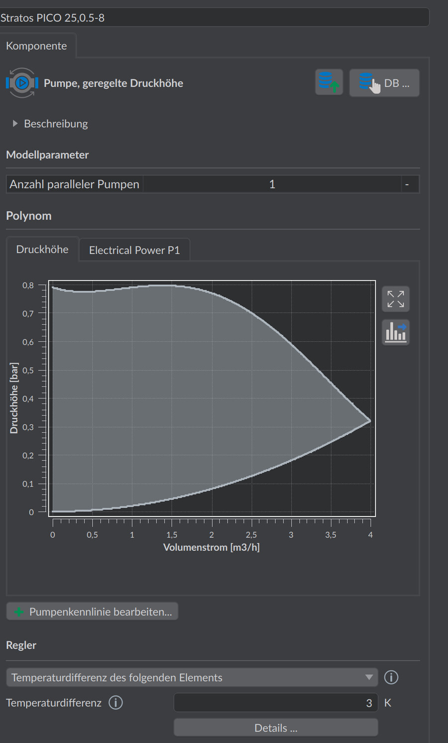
The pressure head is set by the controller assigned to the pump. This pump is the standard model for the central network pump. Controllable quantities are:

• Mass flux – the pump maintains a mass-flux setpoint
• Temperature difference of the following element – e.g. a constant spread across a heat exchanger
• Differential pressure at the worst point – the pump maintains the minimum differential pressure at the hydraulically least favorable consumer in the network (the usual operating mode of network pumps)
• Heating power of the following element – the pump adjusts the mass flux so that a downstream generator delivers a target power
• Outlet temperature on the secondary side – control to the secondary-side outlet temperature of a transfer station

Parameter	Unit	Default	Meaning
Fluid volume	L	1	Fluid volume of the pump
Number of parallel pumps	–	1	Identical pumps in parallel
Lower / upper volume flow limit	m³/s	–	Optional limitation of the operating range

The controlled pump is always power-limited: with an assigned pump curve, its polynomials serve as the limit; without a curve a simplified limitation can be set via the volume flow limits. If the pump reaches its curve limit before the setpoint is met, the setpoint remains unfulfilled – the output quantity VolumeFlowRateExceedance reports the exceedance.

Pump curves

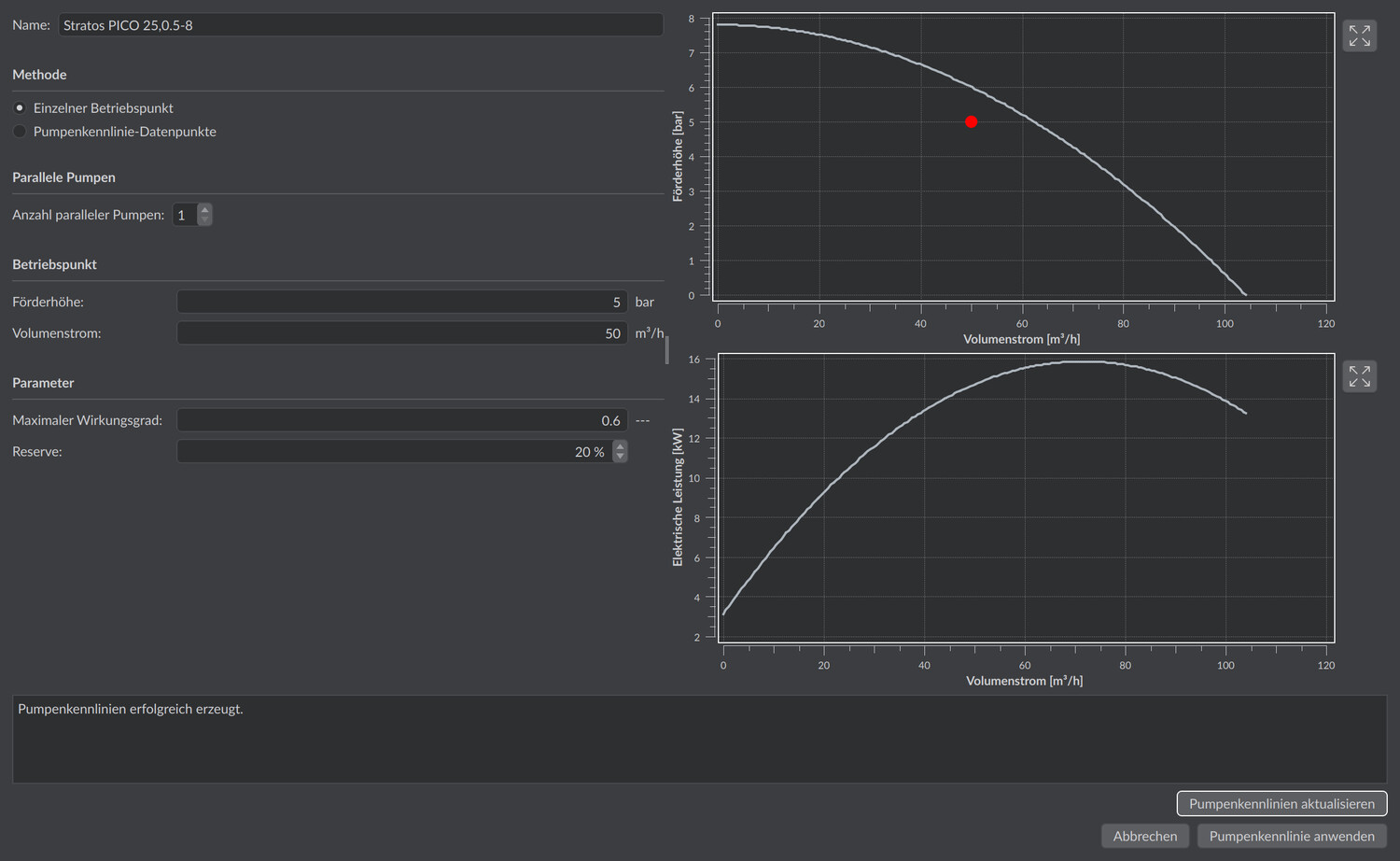
For each pump, curves can be stored as polynomials – the input is entered in the component editor via Edit pump curve…:

• Maximum pressure head $\Delta p_{max}(\dot V)$ as a function of the volume flow – the curve at full speed; it limits the pressure increase, and the root of the polynomial automatically defines the upper volume flow limit
• Maximum electrical power $P_{el,max}(\dot V)$ as a function of the volume flow – the power consumption at full speed

Both polynomials correspond to the datasheet curves of the pump at nominal speed. In addition, lower and upper volume flow limits as well as the volume flow at the best efficiency point can be stored.

Efficiency and electrical power

The electrical power at the operating point follows from the hydraulic power and the overall efficiency (for parallel pumps computed per individual pump and multiplied by the number):

$P_{el} = \frac{\dot V \cdot \Delta p}{\eta}$

For the efficiency $\eta$ the following order of precedence applies:

1. Without a pump curve the constant pump efficiency from the parameters is used.
2. If, in addition to the curve, a constant efficiency > 0 is entered, it takes precedence.
3. If a curve is assigned and no constant efficiency is set, the efficiency is computed as a function of the operating point from the two curve polynomials.

Operating-point-dependent efficiency from the curves

The current operating point $(\dot V, \Delta p)$ of a speed-controlled pump usually lies below the maximum curve – the datasheet curves alone do not provide an efficiency there. The model therefore uses the affinity laws: with a change in speed, an operating point moves along a parabola through the origin, on which the efficiency is approximately constant.

1. Through the operating point, the parabola $\Delta p = a \cdot \dot V^2$ with $a = \Delta p / \dot V^2$ is placed (iso-efficiency parabola).
2. Its intersection $\dot V^*$ with the maximum pressure head curve $\Delta p_{max}(\dot V)$ is determined numerically – this is the corresponding operating point at full speed.
3. There, both datasheet curves are defined, and the efficiency results as:

$\eta = \frac{\dot V^* \cdot \Delta p_{max}(\dot V^*)}{P_{el,max}(\dot V^*)}$

4. According to the affinity laws, this efficiency also applies to the actual (speed-reduced) operating point and enters into $P_{el}$.

Thus efficiency and electrical energy depend directly on both polynomials: the pressure head polynomial determines where the reference point $\dot V^*$ lies, the power polynomial the power consumption there. With curves from the datasheet, the simulation thus delivers realistic part-load efficiencies and annual electricity quantities of the pump; the constant efficiency, by contrast, is a simplification for early planning phases.

With reverse flow the electrical power is zero. Via the optional parameter Fraction of motor losses to the fluid you can define which portion of the loss power is fed to the fluid as heat (wet-runner vs. dry-runner).

Notes

• Pumps are hydraulically active but thermally passive (no heat exchange type); only the set fraction of the motor losses heats the fluid.
• Suggestions for suitable pumps from the database are provided by the pump sizing in the steady-state calculation.

Related topics

• Controllers
• Results of the steady-state calculation
• Component reference