False-Color Display
Show temperatures, volume flows and pressure losses from the network simulation as false colors directly in the 3D scene
Overview
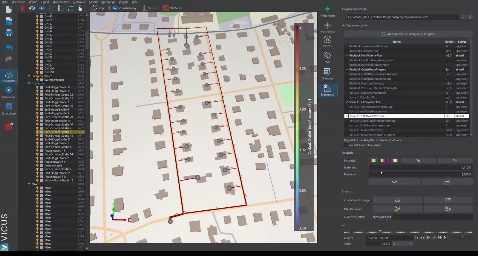
The false-color display colors the heat network in the 3D scene according to the results of the dynamic simulation: temperature, volume flow, pressure loss or heat loss of every route is visualized through a color scale – for either supply or return, at any output time of the simulation. Quantities that relate to flow additionally show arrows in the flow direction. Several configurations can be saved as named views and stored with the project.
Opening
Button  Interactive results in the main toolbar. A completed simulation is a prerequisite; the result files are located in the folder
 <projectname>/results/ next to the project file. In the vertical toolbar to the right of the 3D scene, the  False color view is then active.
Configured Views
The table Configured views lists all saved false-color configurations with the columns Quantity, Unit and Time point. A double-click on a view reads in the result data and displays it in the scene. The status symbol in front of each view indicates:
| Status | Meaning |
|---|---|
| Up to date | The read-in data matches the result files. |
| Reload | The result file has changed (e.g. a new simulation run) – a double-click reloads it. |
| Missing | The required result file was not found. |
You manage the views via the buttons above the table:
| Button | Function |
|---|---|
| + | Add a new configured view from a template |
| Save | Update the selected view with the current configuration |
| Copy | Copy the current configuration into a new view |
| − | Remove the selected configured view |
If the current setting differs from the saved view, the note Configuration differs from saved view appears. All views are stored with the project.
Creating a New View
The + button opens the dialog Create new false-color view. In the quantity selection, you filter the available quantities via the field Filter by quantity name…, or use Show only available to hide all quantities for which no result file exists. Under View name you assign a unique name. Which quantities are available depends on the outputs written during the simulation; with multiple networks the network name is prefixed to the quantity.
Each quantity exists separately for supply and return (e.g. Supply - Temperature):
| Quantity | Unit | Display |
|---|---|---|
| Mass flux | kg/s | Pipe coloring with flow arrows |
| Volume flow | m³/h | Pipe coloring with flow arrows |
| Velocity | m/s | Pipe coloring with flow arrows |
| Pressure difference | Pa | Pipe coloring (absolute values) |
| Pressure gradient | Pa/m | Pipe coloring |
| Pressure | bar | Pipe coloring |
| Operating pressure | bar | Pipe coloring; the gauge pressure including the geodetic component |
| Pressure exceedance | bar | Pipe coloring; amount by which the nominal pressure rating of the pipe is exceeded |
| Temperature | °C | Pipe coloring |
| Heat exchange temperature | °C | Pipe coloring |
| Heat loss | kW | Pipe coloring (absolute values) |
Color Scale and Value Range
| Option | Meaning |
|---|---|
| Color scale | Selection of the color gradient scale used for the coloring |
| Range: Min / Max | Lower and upper limit of the color scale, in the unit of the displayed quantity |
| Hide when: < / > | Objects whose value lies below or above the threshold are hidden in the scene |
| Local min/max | Sets the range to the minimum/maximum of the current time point |
| Global min/max | Sets the range to the minimum/maximum of the entire time series |
The associated color legend is shown in the 3D scene.
Time Point and Animation
The time slider below the settings selects the displayed time point from the simulation’s output times. Date and time are shown, as well as the relative time since the start of the simulation in h. With the playback button, the display runs as an animation over the time series; playback speed and fast forward/rewind can be adjusted.
Analysis Tools
The Analysis area supports targeted evaluation:
| Function | Meaning |
|---|---|
| Jump to time: at maximum value / at minimum value | Jumps to the time point of the largest or smallest value of the entire time series |
| Find object: with maximum value / with minimum value | Highlights the object with the largest or smallest value at the current time point |
| Current selection: | Shows the numeric value of the object selected in the scene at the current time point |
Notes
- If the project was changed after the simulation run or newer result files exist, the status symbol of the view indicates this – the data can be reloaded with a double-click.
- Pressure and heat-loss quantities are displayed as absolute values so that supply and return are colored comparably.
Practical tip
For assessing the network, the extreme time points are the most informative. With Jump to time: at maximum value you immediately find the design situation – for example the coldest operating point or the highest pressure difference – and Find object: with maximum value directly highlights the critical route. Use Global min/max for the value range so that the color scale stays comparable throughout the entire animation.