Transfer station

Overview

The transfer station (district sub station) is the detailed consumer model: a counter-flow heat exchanger with limited transfer capacity and a realistic representation of the secondary side (building heating). Unlike the simple heat exchanger, it can only deliver the required heat flux when the temperature conditions allow it – it is thus the correct model for undersupply scenarios, lowered network temperatures and networks with building-specific differing spreads.

How it works

Transfer capacity (UA value)

The transfer capacity of the station is determined from the design values:

$UA = \frac{\dot Q_{nom}}{\Delta T_{log,nom}}$

The logarithmic temperature difference at the design point $\Delta T_{log,nom}$ is the central quality parameter of the station: a smaller value means a larger, more efficient heat exchanger – the station manages with a smaller temperature gap between network and building and achieves lower network return temperatures. Typical values of modern stations are 5–10 K.

If the design temperatures of both sides are known, $\Delta T_{log,nom}$ for the counter-flow heat exchanger can be computed directly. At the warm end the network supply faces the building supply, at the cold end the network return faces the building return:

$\Delta T_{log,nom} = \frac{\Delta T_A - \Delta T_B}{\ln\!\left(\Delta T_A / \Delta T_B\right)} \qquad \text{with} \qquad \Delta T_A = T_{net,SF} - T_{bld,SF}\,, \quad \Delta T_B = T_{net,RF} - T_{bld,RF}$

Example: network 80/55 °C, building heating 70/50 °C yields $\Delta T_A = 10\,\text{K}$ and $\Delta T_B = 5\,\text{K}$, hence $\Delta T_{log,nom} = (10-5)/\ln(10/5) \approx 7.2\,\text{K}$. If both temperature differences are equal, then $\Delta T_{log,nom} = \Delta T_A = \Delta T_B$.

Secondary side from the heating curve

The secondary side (building heating) is determined from the heating curve of the building:

• Secondary supply setpoint $T_{SF,sec}$ = supply temperature of the heating curve at the current outdoor temperature
• Secondary spread $\Delta T_{sec}$ = temperature difference of the heating curve (for a constant building demand: its constant spread)
• Secondary return: $T_{RF,sec} = T_{SF,sec} - \Delta T_{sec}$
• Secondary mass flux: $\dot m_{sec} = \dot Q_{Bld} / (c_p \cdot \Delta T_{sec})$

With these boundary conditions the model solves the counter-flow heat exchanger analytically and delivers the actually transferred heat flux as well as the outlet temperatures of both sides. The primary-side mass flux is adjusted by the consumer’s control so that the transferred heat flux matches the building demand – as far as the transfer capacity and the network supply temperature allow.

Minimum modulation

If the required heat flux falls below the minimum power $\dot Q_{min} = \dot Q_{nom} \cdot f_{mod,min}$, the station transfers no heat. This allows the cycling behavior of real stations with a modulation limit to be represented. The heat delivery that is thereby lost is made up via the storage term (see below).

Storage behavior

The model keeps an internal storage term $E_{st}$, which sums the difference between delivered and required heat over time:

$E_{st}(t) = \int \left( \dot Q_{delivered} - \dot Q_{required} \right) \, dt$

A negative value is a delivery backlog, a positive one a delivery surplus. The storage level corrects the target heat flux with which the station is operated:

$\dot Q_{target} = \max\!\left(0,\; \dot Q_{Bld} - k \cdot E_{st}\right) \qquad \text{with} \quad k = 0.001\,\tfrac{1}{\text{s}}$

A backlog thus increases the setpoint, a surplus lowers it – the accumulated energy difference is reduced again with a time constant of around 1000 s (≈ 17 minutes).

Physically, the storage term represents the thermal inertia of the building: short interruptions – cycling pauses due to the minimum modulation or briefly too-low supply temperatures – are not lost as energy, but are subsequently made up as soon as the conditions allow it. Over longer periods, the delivered energy sum thereby matches the demand profile; a cycling station with minimum modulation delivers the required power on average. The current storage level is available as the output quantity StoredHeatingEnergy. If the backlog can no longer be reduced because of an insufficient network supply temperature, this shows up in the heat deficit outputs.

Parameters

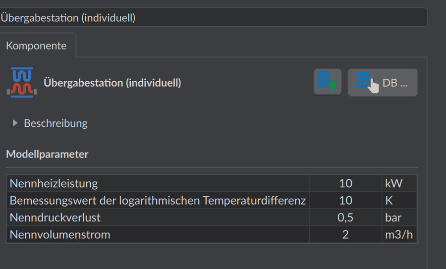
Parameter	Unit	Default	Meaning
Nominal heating power	kW	10	Design power of the station; for the sized variant automatically = connection load of the building
Logarithmic temperature difference	K	10	Design value $\Delta T_{log,nom}$ for the UA value determination
Minimum modulation	–	0	Minimum power as a fraction of the nominal power; below this no heat transfer
Nominal volume flow	m³/h	2	Reference volume flow for the pressure loss; sized variant: automatically from the connection load
Nominal pressure loss	bar	0.5	Pressure loss at the nominal volume flow (quadratic scaling)
Fluid volume	L	3	Fluid volume of the station

Behavior under undersupply

If the network supply temperature drops, the driving temperature gradient in the heat exchanger drops – the station can then no longer fully cover the building demand, even with an increased primary-side mass flux. The transferred heat flux decreases for physical reasons, instead of being extracted unchanged as with the simple heat exchanger.

Persistent deficits are reported as output quantities:

Quantity	Meaning
RequiredBuildingHeatFlux	Heat flux required by the building
HeatDeficitAbsolute	Non-deliverable heat flux [kW], as a time average, as soon as the delivery lies below 95 % of the requirement for longer than 30 minutes
HeatDeficitRelative	Deficit relative to the nominal heating power
OutletTemperatureSecondary / -Setpoint	Achieved vs. required secondary supply temperature
InletTemperatureSecondary	Secondary return temperature
StoredHeatingEnergy	Level of the internal storage term [kWh]: accumulated difference between delivered and required heat

What you need to watch out for: heating curve and network supply temperature

The model stands or falls with a correctly set heating curve per building – it defines the secondary setpoint against which the heat exchanger works:

• The network supply temperature must lie above the secondary supply setpoint – and by at least the order of magnitude of the logarithmic design temperature difference. If, for example, the heating curve requires 70 °C at −12 °C outdoor temperature, but the network delivers only 72 °C, a station sized with $\Delta T_{log,nom} = 10\,\text{K}$ cannot cover the demand: a permanent deficit arises that lies not in the network but in the parameterization.
• After the simulation, check the quantities HeatDeficitAbsolute and OutletTemperatureSecondary against the setpoint: systematic deviations already at mild outdoor temperatures indicate an unsuitable heating curve, deviations only on the coldest days indicate an actual capacity or temperature problem of the network.
• A too optimistically (small) chosen logarithmic temperature difference feigns a too-capable heat exchanger – use datasheet values of the planned stations where available.

Related topics

• Consumer model selection
• Simple heat exchanger
• Heating curves
• Editing building demands