Detailed transfer stations & lowering the supply temperature

District heating network, part 6: configure detailed transfer stations and lower the supply temperature

Overview ▶ 0:08

District heating network for configuring detailed transfer stations — Configuration of more detailed transfer stations that consider the secondary side

This tutorial demonstrates how to model a more detailed transfer station. Unlike the simple variant, the secondary side of the transfer station is taken into account in the heat transfer. With this model, you can better assess what happens when the network supply temperature is lowered, and undersupply is represented more realistically.

Replacing the transfer station ▶ 0:48

Replacement of the simple house transfer station with the detailed variant from the database

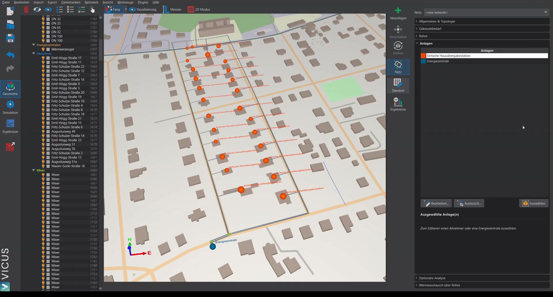
Select the entry Simple house transfer station and click Replace.
Use the predefined database entry House transfer station — best to create a copy so that the entry can be edited.
Select and assign.

Control valve of the detailed transfer station ▶ 1:22

Control valve regulates on secondary-side supply temperature instead of a fixed temperature difference — Detailed transfer station: the control valve regulates on the secondary-side supply temperature

In the system editor, the difference becomes apparent: the control valve now regulates no longer on a fixed temperature difference, but on the supply temperature of the secondary side. This corresponds to the control scheme actually used in district heating networks.

Logarithmic temperature difference ▶ 1:53

Logarithmic temperature difference calculated from primary and secondary side — Logarithmic temperature difference: calculated from supply/return temperatures on both sides (here 9 K)

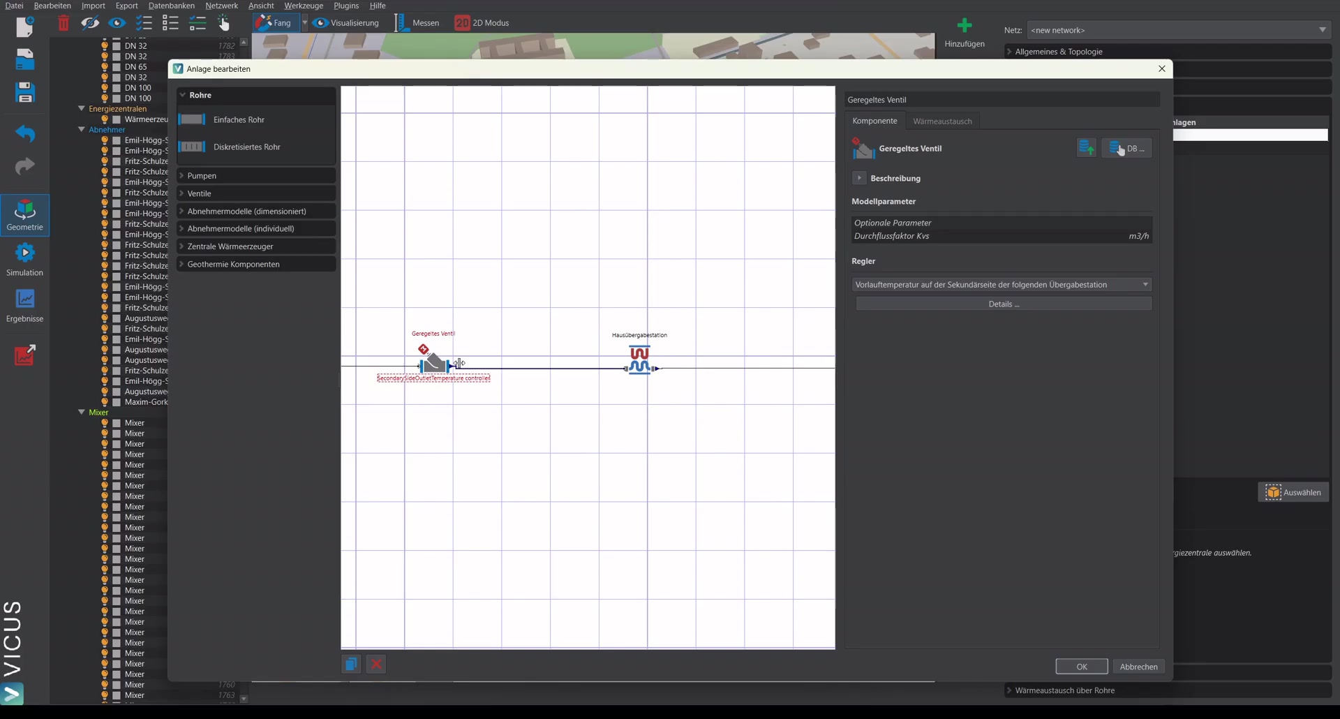
The transfer station has a pressure loss (e.g. 0.5 bar) and a logarithmic temperature difference. This is calculated from:

The supply temperature from the network (primary side)
The return temperature from the transfer station (primary side)
The supply temperature of the building (secondary side)
The return temperature of the building (secondary side)

Note: The smaller the logarithmic temperature difference, the larger the heat exchanger must be. With larger spreads in the network and a larger gap between network supply and building supply, larger logarithmic temperature differences arise — and thus a smaller heat exchanger.

For the example with 78 °C network supply, 70 °C/55 °C building supply/return, a logarithmic temperature difference of 9 Kelvin results.

Simulation with detailed transfer station ▶ 4:28

Simulation over 14 days with detailed transfer station — Simulation with detailed transfer station: results after 14 days of simulation time

After the 14-day simulation, the results show:

Heating power and temperature difference ▶ 4:53

Heating power and slightly fluctuating temperature difference of the transfer stations — Heating power and temperature difference: slight fluctuation due to control on the secondary-side supply temperature

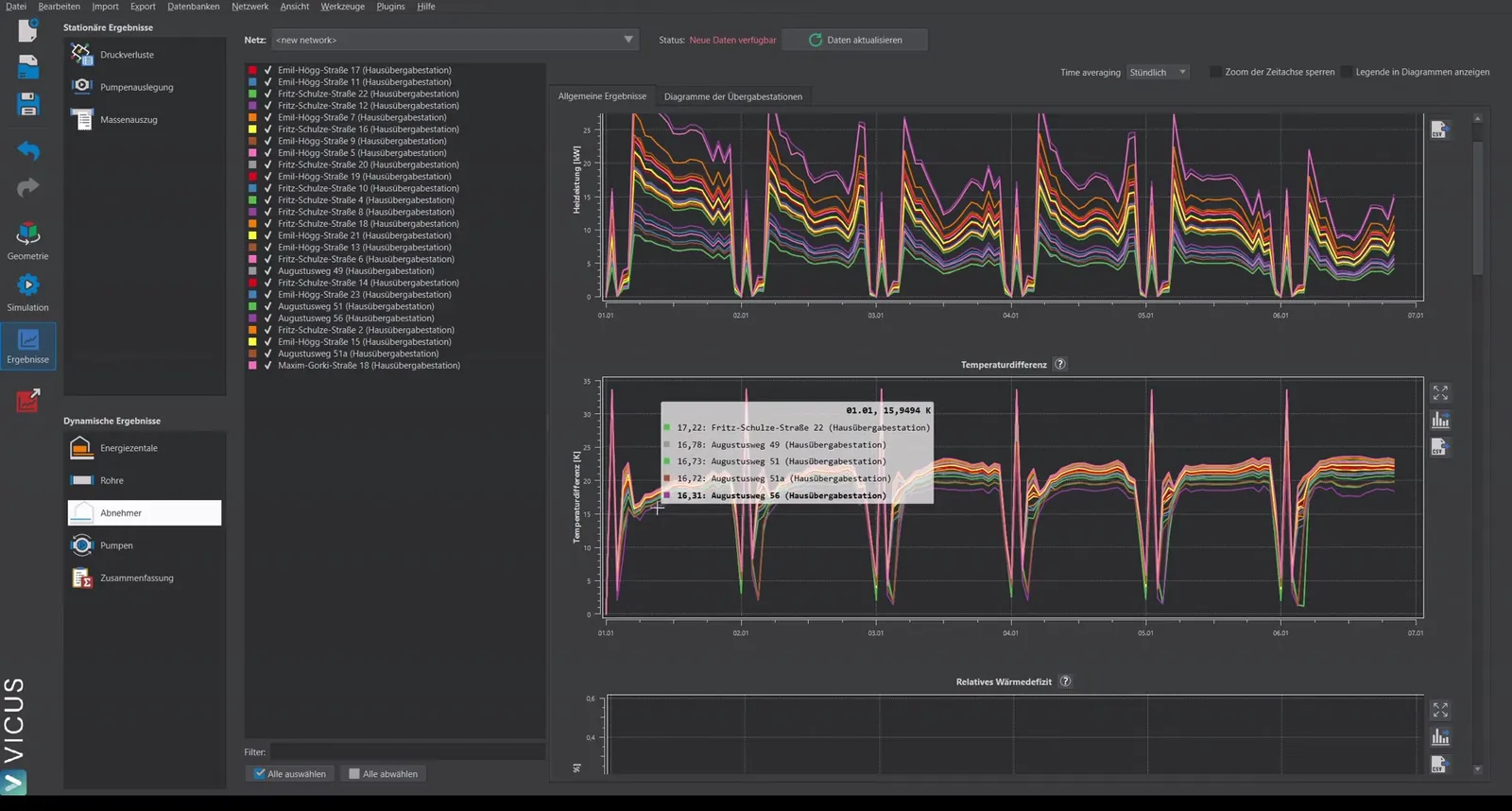
The heating power of the transfer stations is displayed as usual.
The temperature difference is no longer exactly 15 Kelvin but fluctuates slightly. This is because the control is no longer on a fixed temperature difference, but on the secondary-side supply temperature.

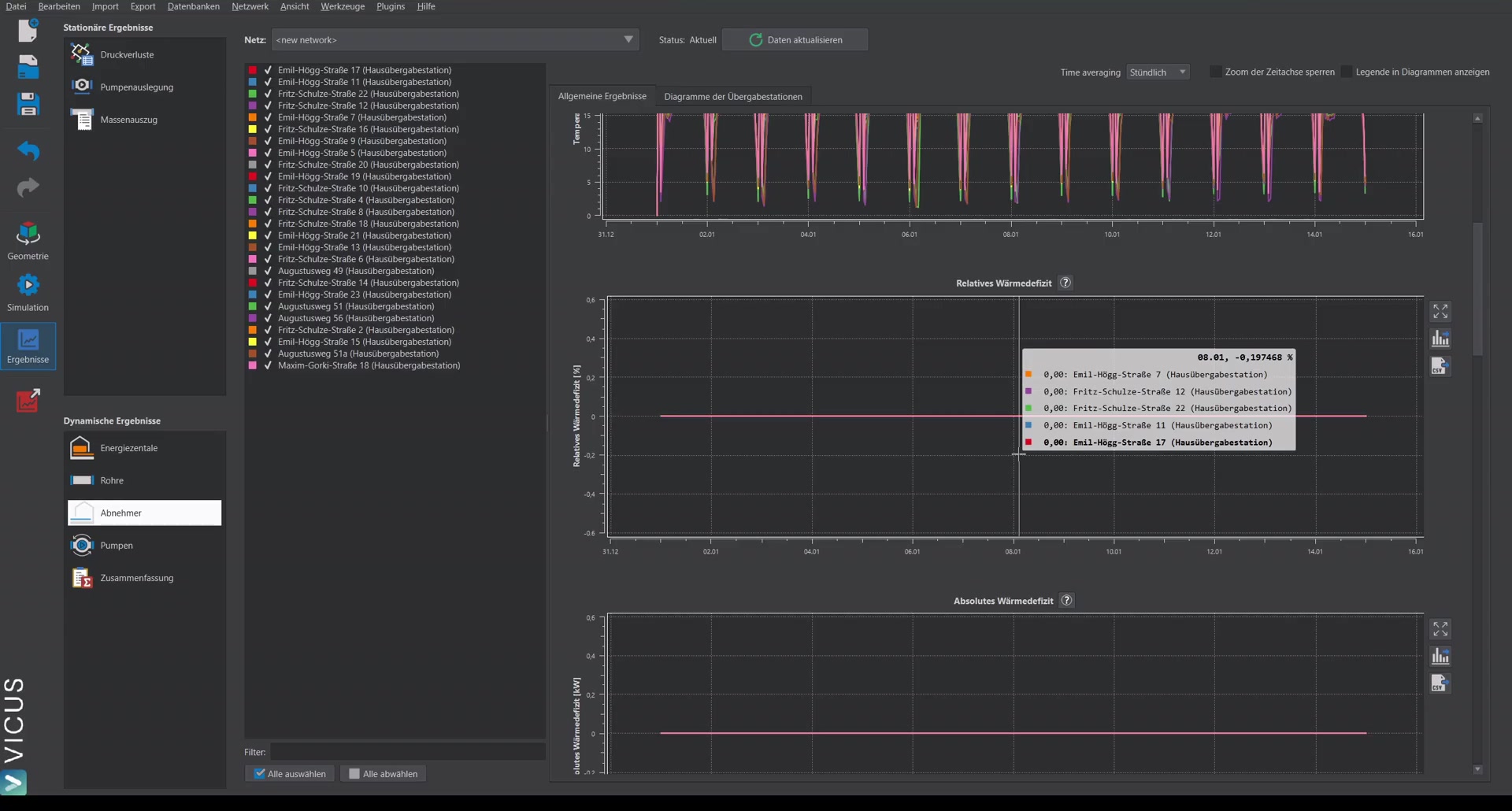
Heat deficit ▶ 5:30

Relative and absolute heat deficit at 80 °C network supply — Heat deficit: at 80 °C network supply the deficit is 0 % — demand is fully met

Two new outputs are available:

Relative heat deficit: Indicates by what percentage the building demand cannot be met.
Absolute heat deficit: Gives the absolute difference in kW.

At 80 °C network supply, the heat deficit is 0 % — the demand is fully met.

Temperature display ▶ 6:15

Detailed temperature display with primary and secondary side per consumer — Detailed temperatures: inlet/outlet temperatures on primary and secondary side per consumer

An additional tab shows, for each consumer, the inlet and outlet temperatures on the primary and secondary sides:

Red: Inlet temperature from the network (approx. 78-79 °C)
Blue (solid): Supply temperature secondary side (actual value)
Blue (dashed): Supply temperature secondary side (setpoint)
Light red: Outlet temperature network side
Light blue: Return temperature secondary side

In addition, for each consumer, the heating power of the transfer station is displayed next to the required heat flow of the building. These do not always match exactly — during load peaks, the heating power cannot always be met immediately because the network takes time to ramp up. The detailed transfer station accounts for a storage effect in this regard.