Simulate a passive network & check the hydraulics

Overview

This third part shows how the hydraulic simulation of a passive cold district heating network works. It examines what influence the pressure losses have on the pump control and whether the decentralized circulation pumps are sufficient to run the network.

Checking the decentralized heat pumps

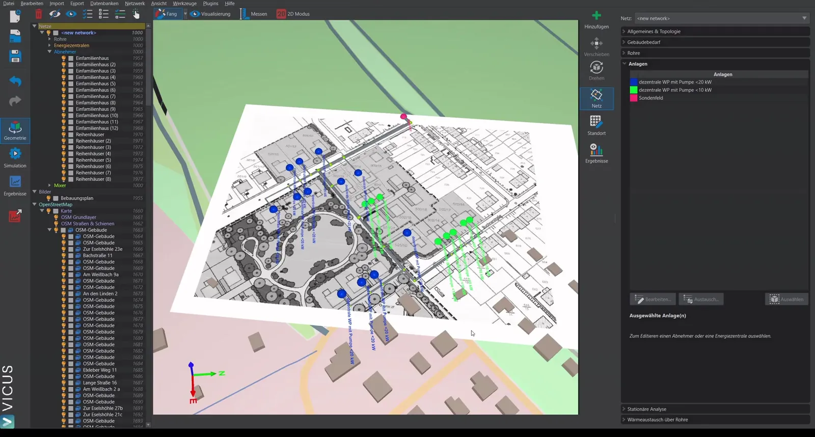
The hydraulic configuration of the decentralized heat pump consists of:

• Circulation pump: A controlled pump that regulates to a temperature difference of 3 Kelvin.
• Heat pump: Passively produces a pressure loss of 0.1 bar.

The volume flow and heating power of the heat pump are automatically set from the stored building data. The associated volume flow is calculated via the 3 Kelvin spread.

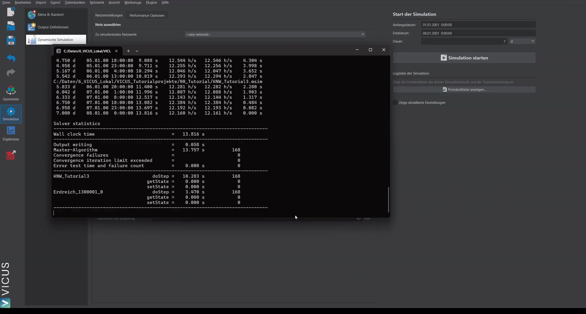
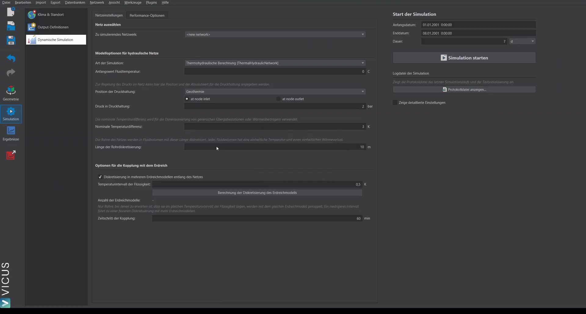
Running the simulation

1. Go to Start simulation.
2. For the first hydraulic check, a short simulation time of 7 days is sufficient.
3. The goal is to check whether the circulation pumps are sufficient to circulate the network.

Evaluating the results

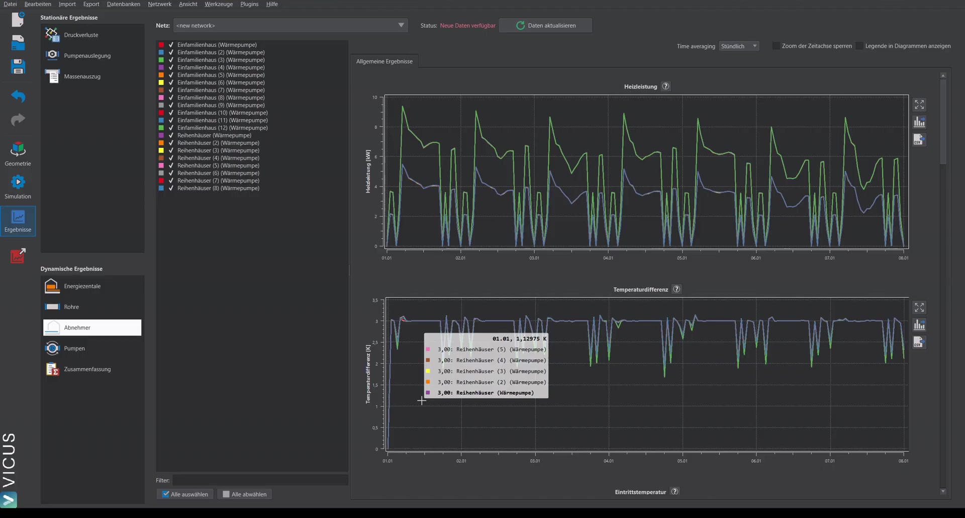
After the simulation, the following quantities are shown in results mode:

• Volume flow and pressure loss at the consumers
• COP of the heat pumps (varies depending on supply temperature and domestic hot-water generation)
• Temperature difference: Should meet the configured 3 Kelvin

Checking the pump operating points

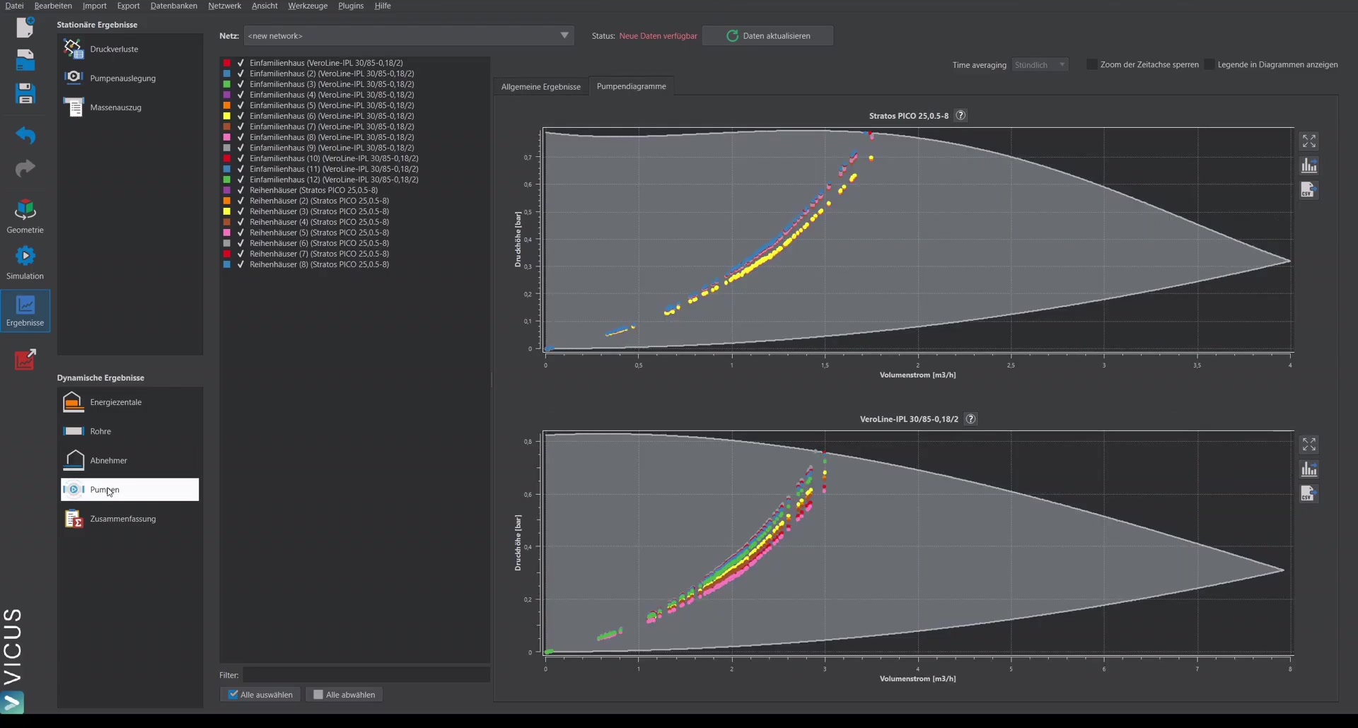
In the Pump diagrams tab, the pump operating points are shown. Because they regulate on a temperature spread, the operating points move along a quadratic curve (not at constant head). The pumps should operate within their operating range.

Testing the effect of higher pressure losses

To evaluate the effect of higher pressure losses, the distributor pressure loss in the borehole field can be increased, for example:

1. Open the plant editor via Databases > Plants.
2. Edit the borehole field and set the distributor pressure loss to, say, 0.25 bar.
3. Run the simulation again.

Evaluating the impact

With increased pressure losses, the following is observed:

• The temperature difference is slightly exceeded (above 3 Kelvin) because the pumps reach their limits.
• The operating points move at most along the pump curve.
• A lower mass flux than required results, which manifests as a higher temperature difference.

This effect demonstrates the correct feedback of the installed pump on the network in the dynamic simulation. For a passive network, it is important to carefully match the pump capacity to the network pressure losses.

Video tutorial