Pipes

Overview

Two model types are available for pipes inside a plant; they differ only in how they represent the thermal behavior. In both cases the pressure loss is computed identically from pipe friction. The pipe properties (inner diameter, roughness, wall structure, insulation) come from the pipe assigned from the pipe database.

Simple pipe

The simple pipe represents the pipe section as a single mixed fluid volume with a uniform temperature. It is suitable for short pipe sections inside a plant where the temperature distribution along the length does not matter.

Parameter	Unit	Default	Meaning
Pipe length	m	100	Length of the pipe section
Number of parallel pipes	–	1	Identical pipes in parallel; the mass flux is split evenly among them

Discretized pipe

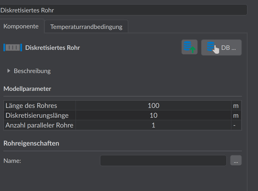
The discretized pipe subdivides the fluid volume along the pipe length into segments and thus represents the temperature distribution within the pipe and the travel time of temperature fronts. It is the correct model when transport delays and cooling-down processes are relevant – for example with long connection lines or in the dynamic simulation. The routes of the heat network itself are also represented as discretized pipes in the simulation.

Parameter	Unit	Default	Meaning
Pipe length	m	100	Length of the pipe section
Maximum discretization length	m	10	Maximum length of a segment; the pipe is automatically subdivided into segments of this maximum length
Number of parallel pipes	–	1	Identical pipes in parallel

Each segment is computed as its own balance volume: a smaller discretization length increases the accuracy of the temperature distribution, but also increases the number of state variables and thus the computation time.

Pressure loss calculation

Both pipe models compute the friction pressure loss according to Darcy-Weisbach, where the friction factor $\lambda$ for laminar and turbulent flow is determined from the Reynolds number and the relative roughness via the Colebrook equation:

$\Delta p = \lambda(Re, k/d_i) \cdot \frac{L}{d_i} \cdot \frac{\rho}{2} \, v \, |v| \qquad \text{with} \qquad v = \frac{\dot m}{\rho \cdot A}$

Here $d_i$ is the inner diameter and $k$ the roughness from the pipe database, $L$ the pipe length and $A$ the flow cross-section. The temperature-dependent viscosity of the fluid enters into the Reynolds number. For parallel pipes, the mass flux is divided by the number of pipes before the calculation.

Heat exchange

Both pipe models support the heat exchange types none (adiabatic), constant temperature and time-dependent temperature. For the simple pipe, the heat flux through the pipe wall is determined from the difference between the (uniform) fluid temperature and the ambient temperature; for the discretized pipe this is done segment by segment – only this way does a realistic cooling-down profile arise along the length.

Notes

• The U-value for the heat losses results from the wall structure and the insulation of the assigned database pipe.
• For representing the pipe installation inside a building (including fittings) there is the dedicated component Building internal installation.

Related topics

• Pipes (database)
• Heat exchange types
• Component reference