Heat pumps

Overview

The heat pump model computes the coefficient of performance (COP) and the electrical power via a biquadratic polynomial from evaporator and condenser temperature, which can be fitted to manufacturer data. There are two integration variants:

• source side (heat pump source side) – a consumer model: the heat pump sits at the building, its evaporator is part of the network. It extracts heat from the network and raises it to the temperature level of the building heating. Typical applications: consumers in cold district heating (5GDHC) as well as booster heat pumps in low-temperature networks whose supply temperature is not sufficient for heating or domestic hot water of individual buildings.
• supply side (heat pump supply side) – a model for the energy plant: the heat pump feeds into the network as a central generator, its condenser is part of the network. It obtains the source heat from outside (e.g. geothermal energy, waste heat).

COP calculation

The COP is computed from the mean temperatures of the evaporator ($T_E$) and the condenser ($T_C$), each in Kelvin:

$COP = c_0 + c_1 T_E + c_2 T_C + c_3 T_E T_C + c_4 T_E^2 + c_5 T_C^2$

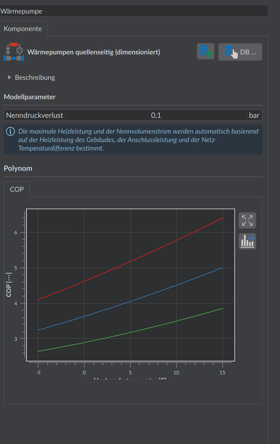
The coefficients are stored in the component editor as a COP polynomial and can be fitted from datasheet characteristic maps (COP at various source/sink temperatures). The default coefficients describe a typical brine/water heat pump (e.g. COP ≈ 5.8 at a 10 °C source and a 35 °C sink temperature).

Operating limits of the model:

• There must be at least 4 K between the condenser and evaporator temperature, otherwise the heat pump switches off.
• If the polynomial yields a COP ≤ 1 (operating point outside the characteristic map), the heat pump likewise switches off.

Electrical power and evaporator power follow from the energy balance:

$P_{el} = \frac{\dot Q_{cond}}{COP} \qquad\qquad \dot Q_{evap} = \dot Q_{cond} \cdot \frac{COP - 1}{COP}$

Heat pump, source side (consumer)

This variant is used in consumer plants – in cold district heating as a regular transfer to the building or as a booster heat pump. The condenser power is the current heating demand of the building, limited by the maximum heating power. The condenser temperature follows from the heating curve of the building (temperature level of the heating system). The evaporator power $\dot Q_{evap}$ is extracted from the network – that is, the building demand minus the electrical share.

For a negative building demand (cooling case) the model works as passive cooling: the heat pump is off, and the cooling load is fed to the network directly as heat – the usual summer behavior in cold district heating networks.

Parameter	Unit	Default	Meaning
Maximum heating power	kW	–	Upper limit of the condenser power; for the sized variant automatically from the building demand
COP polynomial	–	default coefficients	Coefficients $c_0 \dots c_5$
Nominal volume flow	m³/h	2	Reference volume flow for the pressure loss; sized variant: automatically from the connection load
Nominal pressure loss	bar	0.5	Pressure loss at the nominal volume flow (quadratic scaling)
Fluid volume	L	3	Fluid volume (network side, evaporator)

Heat pump, supply side (central generator)

This variant is used in the plant of the energy plant. As a central generator, the heat pump heats the network to the supply setpoint of the heating curve of the energy plant:

$\dot Q_{cond} = \dot m \, c_p \, (T_{SF,target} - T_{in})$

limited by the maximum heating power. The evaporator temperature (heat source) is prescribed as a boundary condition – constant or as a time series via the Heat exchange tab. A heating curve is required.

Parameter	Unit	Default	Meaning
Maximum heating power	kW	–	Upper limit of the condenser power
COP polynomial	–	default coefficients	Coefficients $c_0 \dots c_5$
Nominal volume flow	m³/h	2	Reference volume flow for the pressure loss
Nominal pressure loss	bar	0.5	Pressure loss at the nominal volume flow
Fluid volume	L	3	Fluid volume (network side, condenser)

Output quantities

Quantity	Meaning
COP	Current coefficient of performance
ElectricalPower	Electrical power consumption
CondenserHeatFlux	Condenser power (heating power)
EvaporatorHeatFlux	Evaporator power (source heat)
EvaporatorMeanTemperature / CondenserMeanTemperature	Mean temperatures for the COP calculation

From ElectricalPower, seasonal performance factors and electricity costs can be evaluated – see Line charts.

Notes

• Cold district heating: for consumers with a source-side heat pump, the connection load refers to the evaporator power extracted from the network; this is taken into account in the automatic sizing.
• If the network temperature drops sharply in winter, the COP of the source-side heat pumps drops – the electrical power rises. A look at the COP time series of the critical consumers is part of the evaluation of cold networks.

Related topics

• Automatic sizing
• Heat exchange types
• Component reference