Terrain Elevation and Topography in Network Planning
How terrain elevation enters the pressure balance of thermal networks: DTM versus DSM, data sources, vertical datum and the vertical accuracy actually required
Table of Contents
Elevation differences enter the pressure balance of a thermal network directly through : 10 m of elevation difference correspond to roughly 1 bar, 1 m to roughly 0.1 bar. Together with the pressure loss, the topography therefore decides whether the operating pressure limits are met. The underlying data must be a digital terrain model — a surface model produces errors of several metres in built-up areas, and systematically in the wrong direction, because it maps roofs and tree crowns instead of the road surface.
Why Elevation Matters
The geodetic component shifts the entire pressure level of a network section without changing the mass flows. It therefore acts on both bounds of the pressure balance at the same time: at the high point it decides whether the minimum pressure above the vapour pressure is still maintained, at the low point whether the maximum permissible operating pressure is exceeded. The numerical values of these limits and how they are derived are described in Meeting operating pressure limits and are not repeated here.
Three planning decisions follow directly from the elevation situation:
- Location and fill pressure of the pressurization system. The rest pressure must still be sufficient at the highest point of the network; its fill pressure therefore follows from the elevation difference between the pressurization system and the high point.
- Nominal pressure rating of the pipes at the low point. The lowest network point carries the largest static component and determines which pressure rating has to be assumed for the route.
- Location of the index point. The geodetically most unfavourable point is not necessarily the hydraulically most remote one. In hilly terrain a nearby high point can become the governing index point.
DTM, DSM and the Pipe Axis
The three terms are frequently confused in practice, yet they describe different surfaces:
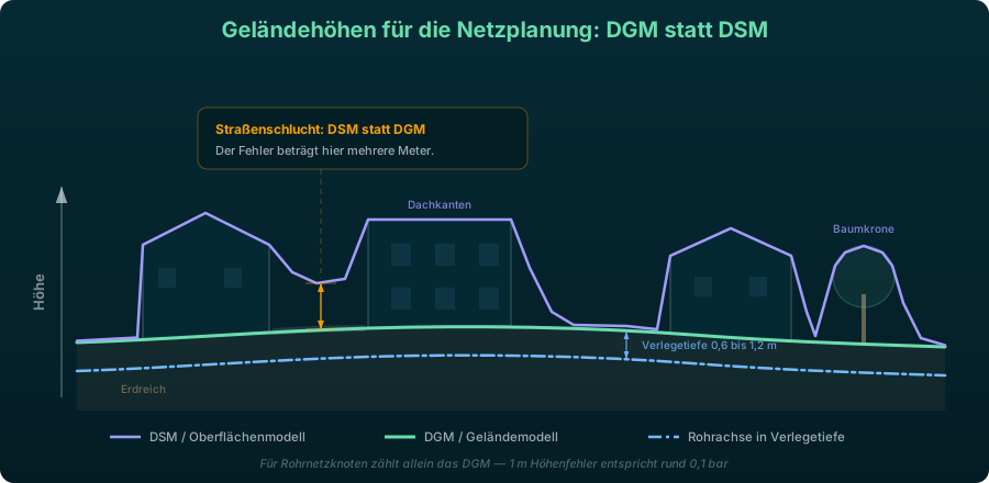
- Digital terrain model (DTM). The bare earth surface without vegetation and buildings. It is derived from LiDAR point clouds by filtering out the ground points. The German survey products are labelled DGM.
- Digital surface model (DSM). The visible surface including vegetation and buildings, called DOM in German usage. In open landscape it is almost identical to the DTM, in built-up areas it is offset by building and tree heights.
- Pipe axis. The line that governs hydraulically. It follows from the terrain elevation minus the burial depth, which for buried networks is typically 0.6 to 1.2 m (see pipe installation and civil works).
Only the DTM is correct for pipe network nodes. In a street canyon a DSM returns the height of the adjacent roof surfaces and therefore a value that sits several metres too high — with a building height of 10 m the error would be of the order of 1 bar.
The deduction of the burial depth, by contrast, is a minor effect: as long as the route runs at a constant depth throughout, it cancels out of every elevation difference. It becomes relevant wherever the burial depth changes, for instance at undercrossings. For the differential pressure at a house connection it is in any case not the pipe axis that counts but the elevation of the transfer station inside the building — for a station in the basement of a building at a high point that is a different value from the terrain elevation at the service line.
Data Sources and Their Accuracy
| Source | Type | Grid spacing | Vertical accuracy | Suitable for |
|---|---|---|---|---|
| Official state survey DGM1 / DGM5 | DTM (LiDAR) | 1 m / 5 m | decimetre range | detailed design, verification of index points |
| National LiDAR-based models via online elevation services | DTM | service-dependent | metre range | preliminary and concept design in Central Europe |
| Copernicus DEM GLO-30 / GLO-90 | DSM, not a terrain model | 30 m / 90 m | vertical datum EGM2008, acquisition 2011–2015 | large-scale terrain overview outside built-up areas |
| SRTM | DSM | — | — | historical reference, superseded for network planning |
The best source is the official state survey. DGM1 and DGM5 are based on airborne LiDAR and reach a vertical accuracy in the decimetre range. They are provided by the surveying authorities of the individual states, where grid spacing and licensing terms have to be enquired.
Online elevation services deliver values sufficient for preliminary design, provided they draw on a national LiDAR-based terrain model for the country in question. For Germany, Austria and the Czech Republic this is the case with services built on a hybrid model structure, and the accuracy is then in the metre range. Which global model underlies the data outside these countries is frequently left undocumented by the providers — outside Central Europe, DTM quality must therefore not be assumed without checking it independently.
Copernicus DEM (GLO-30 / GLO-90) is explicitly a surface model and thus unsuitable for pipe network nodes in built-up areas. It goes back to the WorldDEM/TanDEM-X acquisitions of 2011 to 2015 and is referenced vertically to EGM2008. In street canyons it lies several metres too high, that is precisely where the network nodes are. It remains usable as a large-scale terrain overview outside built-up areas, but not as an elevation source for network nodes.
SRTM is the historical reference from the early days of freely available global elevation data. For network planning it has been superseded by the sources named above.
Vertical Datum and Coordinates
Elevation values always need a statement of what they refer to. Two reference surfaces have to be distinguished:
- Ellipsoidal height. The distance to the reference ellipsoid, as primarily delivered by GNSS measurements and WGS84-based data sets.
- Orthometric height. The distance to the geoid, that is to the physically defined reference surface. Official German heights (NHN, DHHN2016) are orthometric.
The difference between the two surfaces is the geoid undulation. Across the extent of a heat network it changes practically not at all and therefore acts as a constant offset on all nodes.
The practical consequence: for pressure differences only the elevation difference between two points matters. A uniform datum offset across the entire network is therefore uncritical — it cancels out of every difference. What is critical is mixing two sources within one network: if some nodes are taken from an official orthometric DTM and others from an ellipsoidally referenced global data set, a step appears in the elevation line that enters the pressure balance as an apparent elevation difference.
The same applies to horizontal position: within a project a metric coordinate system should be used throughout, in Central Europe usually UTM on ETRS89. Geographic coordinates in degrees are unsuitable for length and route calculations.
How Accurate Does It Have to Be
The conversion factor is the starting point of every accuracy assessment:
where:
- : pressure change caused by the elevation difference [Pa]
- : density of the heating water [kg/m³]
- : gravitational acceleration [m/s²]
- : elevation difference [m]
For water this yields the rule of thumb 10 m ≈ 1 bar, hence 1 m ≈ 0.1 bar. An elevation error therefore translates directly into an error of the calculated pressures — and equally at every bound of the pressure balance.
The accuracy target follows from the planned pressure margin, that is from the distance between the calculated operating point and the respective limit. Rearranged, the rule reads: the tolerable elevation uncertainty in metres is ten times the pressure margin in bar.
| Pressure margin to the limit | Tolerable elevation uncertainty | Sufficient data source |
|---|---|---|
| 1.0 bar | 10 m | any terrain model |
| 0.5 bar | 5 m | LiDAR DTM in the metre range |
| 0.2 bar | 2 m | LiDAR DTM in the metre range, marginal |
| below 0.2 bar | below 2 m | official DGM1 or terrestrial survey |
From this follows the rule of thumb: as long as at least around 0.5 bar of margin to the limit remains at all index points, a LiDAR-based terrain model in the metre range is sufficient. If the margin at a high or low point falls below about 0.2 bar, a single metre of elevation error can flip the result — for that point an official survey or a terrestrial measurement is then required. The effort is small, because it is confined to a few governing nodes and does not concern the whole network.
Typical Sources of Error
Elevation models describe a continuous surface. Wherever the route leaves that surface, the model value deviates from the actual pipe axis:
- Bridges. The DTM usually maps the terrain underneath the bridge, while the pipeline runs inside the structure. The error can amount to the full height of the structure.
- Underpasses and tunnels. The reverse case: the model returns the elevation of the surface passing above, while the pipeline runs below it.
- Excavations and construction states. Models reflect the state at the time of acquisition. After terrain changes, fills or cuts, the value is out of date.
- Embankments and terrain edges. On steep slopes a small horizontal error of the node has a large effect on the interpolated elevation. A lateral offset of a few metres can produce several metres of elevation error on an embankment.
If the elevations come from a surface model, two further systematic errors are added: points that land on rooftops and points in tree crowns. Both sit too high, and both occur preferentially exactly where network nodes are located — at buildings and along tree-lined streets.
Plausibility is best checked not on individual values but on the longitudinal profile of the route. An elevation profile plotted continuously reveals outliers immediately: isolated spikes point to roof or vegetation hits, steps to mixed data sources, a continuous offset to a differing vertical datum. The profile can additionally be verified against a known reference level, such as the elevation of the heating plant.
From Elevation Model to Pressure Diagram
Technically, the path from the elevation model to the pressure diagram runs in five steps:
- Take the elevations of the network nodes from a terrain model — consistently from the same source and in the same vertical datum, so that no datum steps arise.
- Convert to the pipe axis — deduct the burial depth, and at special structures such as bridges, inverted siphons and underpasses enter the actual structure elevation instead of the model value.
- Check the longitudinal profile for plausibility — identify high and low points, clean up outliers and steps, verify the profile against a known reference level.
- Superimpose the geodetic component on the hydraulic pressure profile — the elevation component shifts the pressure level, while the pressure losses from the hydraulic calculation remain unaffected.
- Check the limits at the governing points — minimum pressure at the high point, maximum permissible operating pressure at the low point, keeping the remaining margin above the elevation uncertainty from the previous section.
Topography and Network Structure
Once the elevation difference within the supply area becomes so large that a single pressure level can no longer satisfy both limits simultaneously, this is a question of network structure and no longer of sizing individual components. The usual answers:
- Pressure zones. The network is divided into elevation bands so that each zone stays within its own pressure limits.
- Booster station. Instead of generating the entire pressure loss centrally, pressure is boosted at the periphery. This lowers the pressure level in the central network and allows a lower nominal pressure rating there.
- Network separation via heat exchangers. Hydraulic decoupling of two circuits is the most robust remedy against excessive static pressures with large elevation differences; the secondary circuit receives its own pressurization system. The price is an exergy loss, which is kept small through the lowest possible temperature approach.
- Location of the pressurization system. The pressurization system is preferably arranged such that its rest pressure reliably supplies the high point without overloading the low point. In steeply sloping terrain the location is no longer a free choice but follows from the elevation profile.
- Venting and draining. The positions of the operating valves follow directly from the longitudinal profile: venting at all high points, draining at all low points. Both have to be fixed during route planning already, because chambers have to be provided for them.
Terrain elevation in VICUS Districts:
The elevations of the network nodes are queried from an online elevation service and assigned to the nodes of the active network. They then enter the pressure profile and the network report as the geodetic component, which plots the geodetic height over the route length alongside the operating pressure and the pressure loss line. The data basis is the Mapy.com Elevation API, a hybrid model: a global elevation model worldwide, but national LiDAR-based datasets for the Central European countries. For projects in Germany, Austria and the Czech Republic the service therefore returns terrain elevations from a DTM in the metre range — accurate enough to capture the high and low points of a route and the order of magnitude of the static pressure, but not a survey. An uncertainty of around 1 m leaves roughly 0.1 bar of uncertainty in the pressure level.
Further reading: Meeting operating pressure limits — the limits against which the elevation profile is checked, Pressure profile and pressure diagram — the representation in which the geodetic component becomes visible, Pipe installation and civil works — burial depth, longitudinal profile and the chamber and valve locations that follow from it.
References and Standards
- AGFW FW 442 — Pressure Maintenance in Hot Water District Heating Networks
- DIN EN 13941 — District Heating Pipes — Design and Installation of Factory-insulated Bonded Pipe Systems
- Nussbaumer, T.; Thalmann, S.; Zaugg, D.; Cueni, M. (2025): Planungshandbuch Thermische Netze. Version 2.0, EnergieSchweiz / Swiss Federal Office of Energy.
- Official surveying authorities of the German states (AdV) — Digital terrain models DGM1 and DGM5
Frequently Asked Questions
What is the difference between a DTM and a DSM?
How accurate do terrain elevations have to be for pressure calculations?
Which elevation counts hydraulically, the terrain or the pipe axis?
Related Articles
What operating pressure, rest pressure, MOP, MIP and the nominal pressure rating mean, why gauge pressure is the working convention, and how the minimum pressure follows from the saturation pressure plus 1.5 bar
Network operating modes in district heating networks: sliding, constant, and sliding-constant operation. Operating principles, advantages and disadvantages compared.
Pressurization systems in thermal networks: open and closed systems, pre-charge pressure from the static height, expansion volume and make-up water
The pressure diagram of a heat network: static pressure, rest pressure and pressure loss, the index point and the minimum differential pressure of 0.5 to 1.0 bar required there
Disclaimer: The content of this page is for general information purposes only and does not constitute legal, planning or engineering advice. All information is provided without guarantee. Despite careful research, VICUS Software GmbH assumes no liability for the accuracy, completeness or timeliness of the information provided. Third-party product names and trademarks are mentioned for informational purposes only and are the property of their respective owners.