Heat network simulation: dynamic and thermo-hydraulic
Annual simulation of pressure, mass flow and temperature
A heat network simulation answers questions that sizing for peak load leaves open: how warm is the water at the last house connection in July? What are heat losses and pump electricity over the year? What happens when a second producer feeds in? A dynamic thermo-hydraulic annual simulation calculates pressures, mass flows and temperatures in coupled form at hourly resolution (8,760 hours) – including control and heat exchange with the ground.
This page describes what district heating simulation is needed for in planning and how it works in VICUS Districts, the district heating software for network design. The methodology itself – equations, pipe models, numerics – is explained in the knowledge article on thermo-hydraulic simulation of district heating networks. The simulation core, the VICUS Solver, builds on more than 20 years of research at TU Dresden.
What a thermo-hydraulic simulation is needed for
Typical planning questions that can only be answered reliably with a time-resolved, coupled calculation.
Temperatures at the end of the network
Which supply temperature still reaches the last consumer in summer at low demand? On long branch lines under part load it drops noticeably due to heat losses and long residence times – an effect only a time-resolved calculation reveals.
Part load and summer operation
Networks are sized for peak load but run at part load for most hours of the year. Mass flows, flow velocities and relative heat losses then behave fundamentally differently from the design case.
Return temperatures
The return temperature is calculated at every substation and in every pipe segment. This shows how return temperature limits or poorly cooling consumers affect the efficiency of heat pumps, solar thermal or waste heat recovery.
Pump control
Differential pressure, temperature difference or index-point control act over the whole year. The simulation reports pump electricity as an annual total rather than a snapshot at the design point.
Storage and multiple heat sources
With several feed-in points, flow directions and mixing temperatures change across the network. Buffer storage in the substations is balanced over time; more detailed storage models can be coupled via FMI 2.0 (FMU).
Cold networks with ground model
In cold district heating, uninsulated pipes and the surrounding soil are part of the energy system. A finite-volume ground model captures heat gains, ground cooling and the long-term behaviour of the soil over the years.
When a steady-state calculation is enough
Steady-state is sufficient
- Pipe sizing for the design case with simultaneity
- Pressure loss, index point and pump sizing
- Branched networks with one producer and conventional temperature levels
- Comparing route variants in preliminary design
Dynamic is required
- Multiple feed-in points, meshed networks, changing flow directions
- Low network temperatures, temperature reduction in existing networks
- Summer part load and supply temperature at the end of the network
- Storage, control strategies, ground coupling (cold district heating)
- Annual figures: heat losses, pump energy, producer shares
In practice the two complement each other: in VICUS Districts the network is first sized in steady state for selected operating points (maximum heating load, part load, specific hours of the year) and then simulated dynamically with the same model. How operating points and operating modes relate is covered in the article on network operating modes.
Heat network simulation workflow in VICUS Districts
Capture the network
Import routes from GIS data (Shape, GeoJSON, GeoPackage) or draw them on an OpenStreetMap, DXF or PDF background. Geodetic heights are set by the built-in terrain model.
Parameterise consumers and producers
Load profiles for space heating and domestic hot water from standard profiles or as an import (CSV, Excel). Heat producers and substations are assembled from a modular component catalogue.
Steady-state pre-sizing
Pipe sizing with simultaneity, pressure loss including fittings and substations, index point and pump sizing for selected operating points.
Dynamic simulation
Thermo-hydraulic simulation over a week or a full year, with control, ground coupling and either the dynamic (segmented) or the simple pipe model.
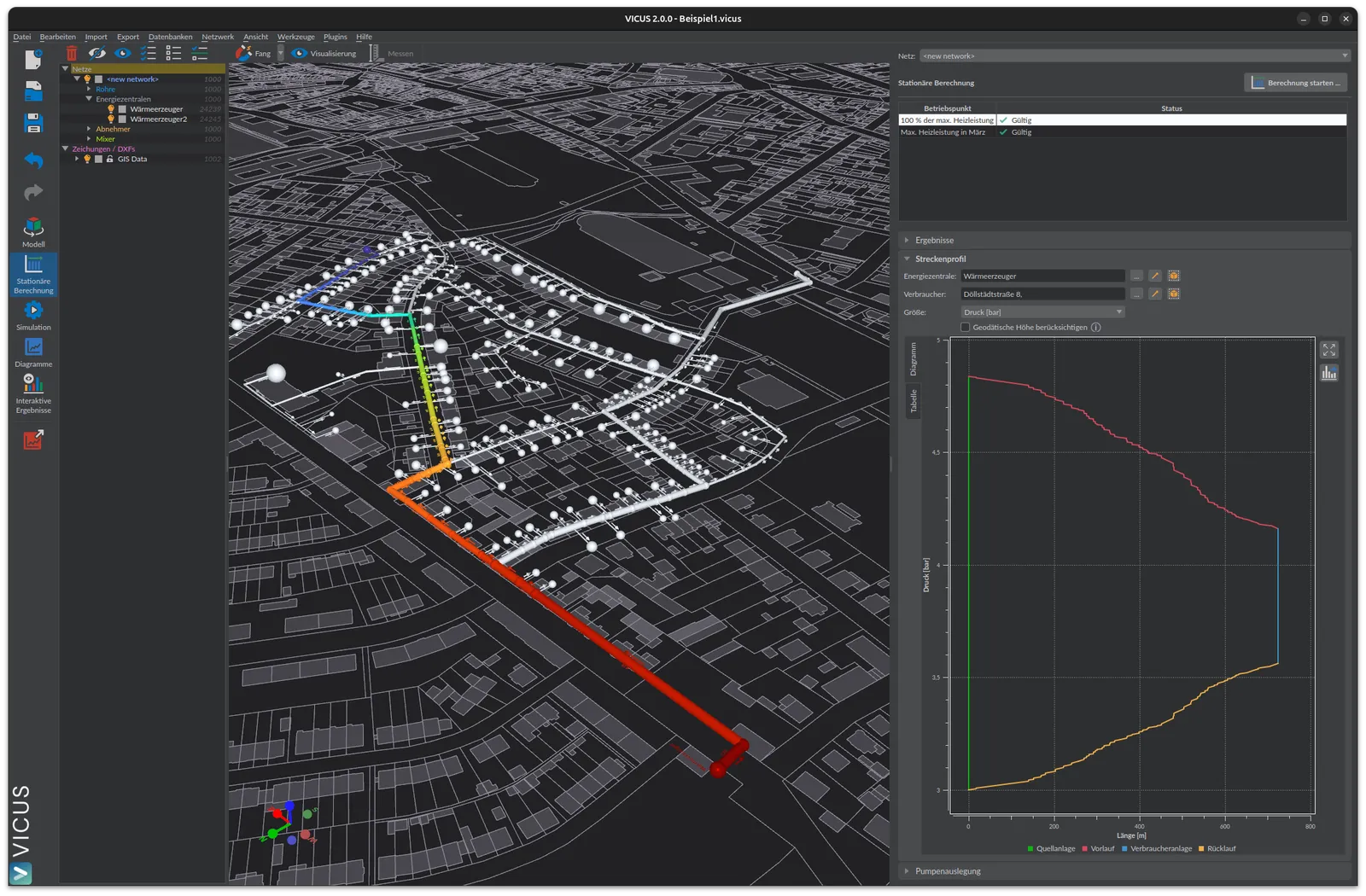
Simulation results
- Supply and return temperatures per node, pipe segment and substation over time
- Mass flows, flow velocities and flow directions – including changing feed-in
- Pressure distribution, index point and route profiles between producer and consumer
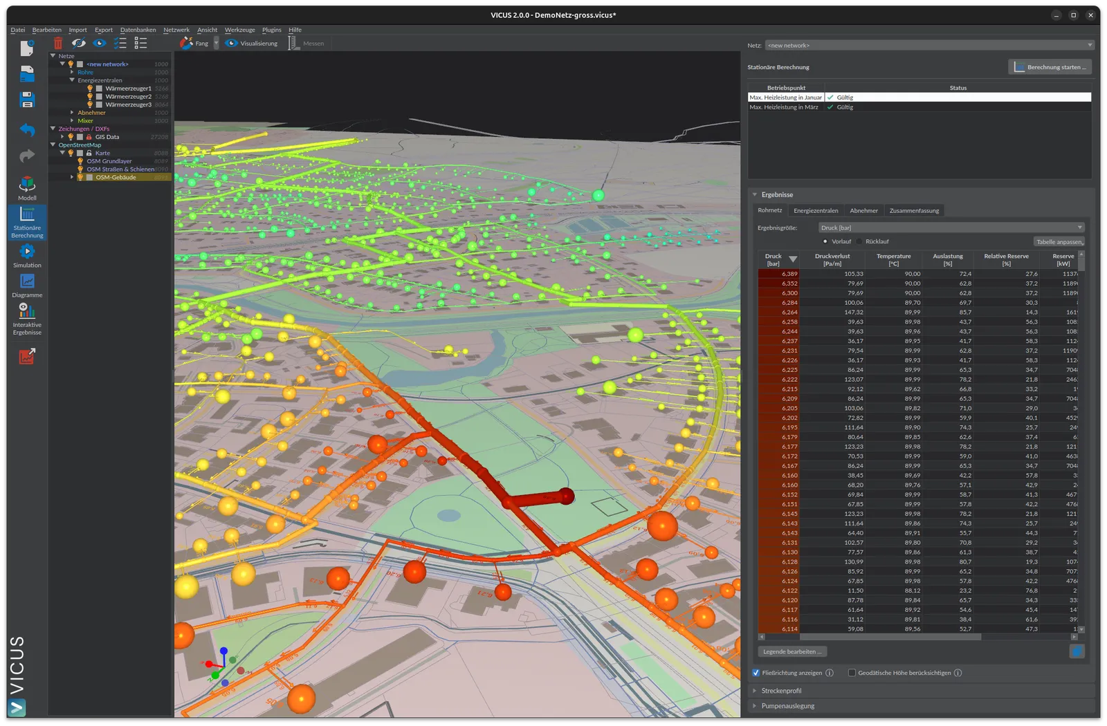
- Network heat losses as hourly values and annual totals
- Peak loads, heat delivered per producer and pump energy
- Colour-coded network plans (PDF, PNG), bills of quantities and GIS export of results
How the pressure profile and network control interact is described in detail in the knowledge base. How the solver couples hydraulics and heat transport numerically is shown in VICUS Solver: the engine behind heat network simulation.
More from our knowledge base
Frequently asked questions
Simulate your own network
In a personal demo we show the annual simulation on an example network – or try VICUS Districts free for 30 days.