Contents
A dynamic building simulation needs a computational core that turns geometry, building components, weather and use into the time history of temperatures and loads. In VICUS Buildings this core is the VICUS Solver, built on more than 20 years of research at TU Dresden.
This article explains how such a core works. The principles apply to practically every dynamic building simulation; where the VICUS Solver makes a specific choice, this is stated. Each section starts with a simple example and then moves on to the method. No background in numerical methods is required. If you want to try the methods yourself, the Solver Lab offers four interactive experiments on time step, stability and grid spacing.
The core idea: bookkeeping of energy
Picture a bathtub with the tap running and the drain open: the water level rises when more flows in than out, and falls in the opposite case. Knowing the inflow and the outflow, you can predict the water level at any later time.
A room works the same way, only with heat instead of water. Inflows are solar radiation, people, equipment and heating; outflows are transmission through the envelope and ventilation. The “water level” is the heat content, i.e. the stored internal energy :
In words: the change of heat content per unit time equals the sum of all inflows minus the sum of all outflows. The solver sets up this one balance for every room and every wall layer and advances it step by step through time.
Why energy and not temperature?
Temperatures cannot simply be added up, energies can. The same kilowatt-hour has very different effects depending on where it is stored:
| Heat capacity | Temperature rise from 1 kWh | |
|---|---|---|
| Room air, 50 m³ | about 60 kJ/K | about 60 K |
| Concrete slab, 10 m² × 20 cm | about 4,800 kJ/K | about 0.75 K |
The energy is the same in both cases; only the temperature change differs, by a factor of 80. This is why the solver balances energy, which can be summed unambiguously, and then computes the temperature from the heat capacity: .
A single room as a worked example
The simplest building model is a single room with heat capacity , connected to the outdoor air through a heat loss coefficient (transmission and ventilation combined, in W/K). Without heating, heat flows out in proportion to the temperature difference:
With this gives the equation that describes the room cooling down:
The time constant expresses how sluggish the room is. After one time constant, about two thirds of the temperature difference to the outdoor air has gone; after three time constants, about 95 %.
Two variants of the same room with W/K show how large the difference can be:
| Heat capacity | Time constant | almost cooled down after | |
|---|---|---|---|
| room air only (50 m³) | 60 kJ/K | 10 minutes | 30 minutes |
| room air with walls, ceiling, screed | 10,000 kJ/K | about 28 hours | about 3.5 days |
One time step by hand
With the sluggish room, a single computation step can be followed directly. It is 20 °C inside and 0 °C outside, and the time constant is 28 hours. The rate of change is then
A step of one hour gives °C. The exact solution is 19.30 °C. The new temperature then yields a new rate of change, the next step is taken, and so on.
This is exactly how a building simulation works: determine the rate of change, take a step into the future, repeat. Everything else in this article is about doing this quickly, stably and accurately for thousands of coupled quantities. In the Solver Lab you can work through this example interactively.
From room to building: the state vector
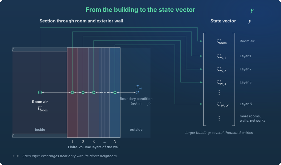
A real building has more than one heat store. Every wall stores heat, and not uniformly: in winter the inside of an external wall is warm and the outside cold. To capture this temperature profile, the solver splits every construction into many thin layers (finite volume elements). Each layer gets its own energy balance.
All quantities that store energy and change over time are collected by the solver in one long list, the state vector :
| Part of | Meaning |
|---|---|
| Rooms / zones | Internal energy of the room air (and moisture, if modelled) |
| Constructions | Internal energy in every layer of every wall, ceiling and floor slab |
| Thermal networks | Energy of the fluid in pipes and components |
The order of magnitude is easy to estimate: 50 components with 30 layers each already give 1,500 entries, plus the rooms. Larger buildings reach several thousand.
For the whole building, the task can then be written in short form:
This is nothing more than the bathtub balance, applied to all stores at once. (“y-dot”, in source code usually ydot) is the list of all rates of change: for every room and every layer, how fast the heat content is currently rising or falling.
How the rates of change are obtained
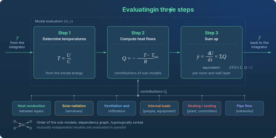
For the single room, the rate of change could be written as a formula. With thousands of coupled stores this is no longer possible. Instead, is assembled afresh at every call, in three steps:
- Determine temperatures: the temperature of every room and every layer is computed from its stored energy.
- Compute heat flows: each sub-model contributes its share, such as conduction between layers, solar radiation through windows, ventilation and infiltration, internal gains, heating and cooling power, or pipe flow.
- Sum up: for every room and every layer, all inflows and outflows are added. The result is the corresponding entry in .
Example: an office on a winter afternoon
For a single room, step 3 might look like this at a given moment:
| Heat flow | Contribution |
|---|---|
| Sun through the window | +300 W |
| Two people and computers | +200 W |
| Transmission through the envelope | −400 W |
| Ventilation | −150 W |
| Heating (thermostat closed) | 0 W |
| Sum = entry in | −50 W |
The room is currently losing 50 W. With an effective heat capacity of 10,000 kJ/K, its temperature therefore drops by just under 0.02 K per hour. This number, for every room and every layer, is what the solver needs for the next time step.
The right order: the dependency graph
The sub-models in step 2 depend on each other, much like trades on a building site: the screed goes in only after the underfloor heating. In the simulation, for example, the window model needs the sun position from the climate model, and the room balance needs the output of the heating model:
Weather data → sun position → radiation on the window → heat gain in the room
The VICUS Solver determines the order automatically using a dependency graph. Each model declares which quantities it needs and which it provides; topological sorting then yields a valid evaluation order. Two cases matter:
- Parallel evaluation: models that do not depend on each other, such as heat conduction in many different walls, are computed simultaneously on several processor cores.
- Loops: a thermostat measures the room temperature and sets the heating valve, the valve determines the heating power, and the heating power changes the room temperature. Models that influence each other in this way are grouped by the solver and solved together iteratively.
Step by step through the year
With , the rate of change of every store is known. Time integration turns this into the course of the year: it moves from to , computes the new state and repeats until the end of the simulation.
The step size is not fixed. The solver adjusts it continuously, much like a driver who goes faster on an open road and slows down before a bend:
- At night, heating in setback mode, little change: large steps, by default up to one hour in VICUS Buildings.
- In the morning the heating starts, a window is opened, a blind comes down: small steps of seconds to minutes until the system settles.
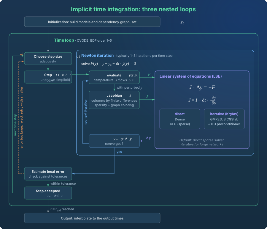
After every step the solver checks whether it was good enough: it estimates the error and compares it with a tolerance (in VICUS Buildings a relative tolerance of by default). If the error is too large, the step is rejected and repeated with a smaller step size; if it is well below what is needed, the next step may be larger.
Result output is independent of this. If you request hourly values, you get them, even though the solver has computed with entirely different steps internally; values are interpolated between computation steps to the output times.
Explicit or implicit
There are two fundamentally different ways to take a time step.
Explicit means: the rate of change is determined at the start of the step and used for the whole step. That was the step by hand in the room example.
Implicit means: the rate of change at the end of the step is used, i.e. at the still unknown new state. The result therefore appears on both sides of the equation and must first be solved for:
The explicit step is simpler and cheaper. The room shows once more why buildings are nevertheless computed implicitly.
Example: the fast room with a large step
This time the room in which only the air stores heat ( = 10 minutes). 20 °C inside, 0 °C outside, a step size of one hour, i.e. six time constants at once:
| after | explicit | implicit | exact |
|---|---|---|---|
| 1 hour | −100 °C | 2.9 °C | 0.05 °C |
| 2 hours | +500 °C | 0.4 °C | 0.00 °C |
| 3 hours | −2,500 °C | 0.06 °C | 0.00 °C |
The explicit method takes the initial cooling rate of 2 K per minute and applies it for 60 minutes. It overshoots far below the outdoor temperature, then even further above it in the next step, and the solution blows up. The implicit method asks instead: which temperature at the end of the step matches the cooling rate at exactly that point? The answer is not exact, but it is physically sensible and stable. With a smaller step it also becomes more accurate.
Here, an explicit method only stays stable if the step is shorter than about two time constants, i.e. shorter than 20 minutes.
Stiff systems
A building contains both room variants at the same time: parts that react within minutes (room air, thin plaster layers) and parts that take days (concrete slabs, screed). Such systems are called stiff. An explicit method must always follow the fastest part, even when that part is hardly changing at all.
A numerical example from the wall: for a layer of thickness made of a material with thermal diffusivity , the explicit method is stable only for
For lime plaster ( m²/s) and 1 cm layers that means at most 100 seconds per step, i.e. more than 300,000 steps for one year. Halve the layer thickness and the time step must drop to a quarter. An implicit method, by contrast, can take steps of up to one hour when little is changing. Each of these steps costs more, but overall the implicit method is considerably faster for buildings. In the Solver Lab you can push past this limit directly by changing time step and grid spacing.
| Explicit | Implicit (default in the VICUS Solver) | |
|---|---|---|
| Rate of change taken at | start of the step | end of the step |
| Equation to solve | no | yes, with Newton iteration |
| Cost per step | low | high |
| Step size limited by | stability (very small for buildings) | accuracy |
| Suitable for buildings | no (too slow) | yes |
CVODE: the default integrator
By default the VICUS Solver uses CVODE from the SUNDIALS suite, an implicit method with adaptive step size based on BDF (Backward Differentiation Formulas). The simplest BDF method (order 1) is exactly the implicit step shown above. Higher orders (up to 5) also take the previous time steps into account, much as a curve through several points describes a trend better than a straight line through two. CVODE chooses step size and order itself. Explicit methods (Euler, Runge-Kutta) are available in the solver as reference and test integrators.
What happens inside an implicit step
An implicit time step consists of three nested levels:
- Time loop (CVODE): chooses the step size and moves from to .
- Newton iteration: solves the implicit equation for the new state , usually in 1 to 3 passes.
- Linear system of equations (LSE): in every Newton pass, one system of equations is solved.
The Newton iteration
The Newton iteration is a method for solving equations that cannot be rearranged directly for the unknown. A familiar example is the square root of 2, i.e. the solution of :
- Start with an estimate, say .
- At this point, draw the tangent to the curve and find where it crosses zero: at .
- Repeat from there: .
After two passes the result is correct to four decimal places (). Each pass replaces the difficult equation with a straight line that is easy to solve.
In the solver, the equation that every implicit step has to solve is:
The tangent is here called the Jacobian , and the correction to the estimate follows from
If all heat flows were linear in temperature, Newton would be finished after one pass, as in the room example. Non-linearity comes from long-wave radiation (proportional to ), temperature-dependent heat transfer and controllers. But since the state from the previous time step is already a very good starting estimate, 1 to 3 passes are usually enough.
The Jacobian
For every pair of state variables, the Jacobian answers a question of the kind: how much does the balance of room A change if the temperature of wall layer B rises slightly? With state variables it has entries:
The VICUS Solver determines these entries by trial: it changes one state variable slightly, evaluates again and checks which balances have changed and by how much. That gives one column of the matrix.
The linear system of equations
With thousands of unknowns, solving is the most computationally intensive part of the simulation. What makes it manageable is a property of the matrix.
Almost all entries are zero
A wall layer exchanges heat only with its two direct neighbours, a room only with the adjoining component surfaces. For a wall with five layers the matrix therefore looks like this (× = non-zero entry, blank = zero):
13 of the 25 entries are occupied. With 30 layers it is 88 of 900, and for a building with several thousand states well under one percent. Such matrices are called sparse, and there are solvers that work only with the occupied entries.
Sparsity also saves effort when building the matrix. If layer 1 is perturbed, only layers 1 and 2 respond; if layer 4 is perturbed, only layers 3 to 5. The two perturbations do not overlap and can therefore be tried at the same time in a single evaluation of . For a wall, three evaluations are enough this way (layers 1, 4, 7, …; then 2, 5, 8, …; then 3, 6, 9, …), regardless of whether it has 10 or 100 layers. This grouping of independent columns is called graph colouring; the VICUS Solver knows the sparsity pattern in advance and applies it to the whole building.
Direct and iterative solvers
There are two kinds of solvers for the system of equations:
- Direct solvers work on the principle of Gaussian elimination from school: eliminate unknowns step by step, then substitute backwards. Technically this is done via an LU decomposition, as a dense variant (Dense) for small systems or a sparse one (KLU) for large ones. The result is exact up to rounding errors.
- Iterative solvers (Krylov methods such as GMRES or BiCGStab) approach the solution step by step. They need less memory and can be faster for very large systems. To make them converge quickly, the system is first conditioned with a preconditioner, such as an incomplete LU decomposition (ILU).
The default in VICUS Buildings is the direct sparse solver KLU. For typical building models it is the most robust choice.
What this means in practice
In day-to-day design work nobody has to configure these methods. Understanding them helps, however, when a simulation takes unusually long. The most common causes follow directly from this article:
- Many small time steps due to switching: a thermostat with a narrow switching differential, or shading that opens and closes frequently, forces the solver into small steps at every switch.
- Very fine discretisation: more layers per component mean more unknowns and therefore larger systems of equations.
- Many Newton passes: strongly non-linear models or abrupt input data worsen convergence, and steps are rejected more often.
Solver settings in VICUS Buildings
The defaults (CVODE, KLU, relative tolerance , maximum step size 1 hour) are almost always the best choice for building simulations. If you want to adjust them, all fields are described in the manual under Solver options. Before changing tolerances, look at the solver statistics: they show whether the time goes into many small steps, into Newton passes or into the linear system.
The VICUS Solver is the computational core of VICUS Buildings; its methodology is documented through the open-source project SIM-VICUS. Background is provided in the articles on dynamic building simulation, on the difference between steady-state and dynamic calculation and on validation standards. How the same computational core solves a district heating network is described in VICUS Solver: the Engine for Heat Network Simulation.
Summary
- The solver keeps books on energy: for every room and every wall layer, the change in heat content equals inflows minus outflows. Together this gives .
- is assembled afresh at every call: determine temperatures, compute heat flows, sum up. The order of the sub-models follows from a dependency graph.
- Computation proceeds in time steps of adaptive size: large when little happens, small during switching events.
- Because buildings are stiff (minutes next to days), the computation is implicit, by default with CVODE. Explicit methods would have to follow the fastest part and would be too slow.
- Every implicit step requires a Newton iteration, and every Newton pass a linear system of equations. The fact that the matrix consists almost entirely of zeros is what makes both fast.
Authors

Dr.-Ing. Andreas Nicolai
Chief Technology Officer
Developer of the solver and 3D engine, with years of experience in numerical simulation and software architecture.

Dipl.-Ing. Stephan Hirth
Lead Developer VICUS Buildings
Algorithms, workflows and GUI of VICUS Buildings – from solver integration to the 3D engine.