Pump Sizing in District Heating Networks
Central vs. decentralised pump concepts: sizing, index-point control and energy demand
Table of Contents
Pump sizing determines whether a district heating network can be run efficiently and economically. The flow rate follows from the network heat output and the temperature spread, while the pump head follows from the pressure losses along the most critical supply path. In a well-designed network, pump electricity consumption stays at 1—2 % of the transported heat. With unfavourable dimensioning, especially in low-temperature networks with small temperature spreads, it can climb to 5—10 % and put the economics of the whole project at risk.
Online calculator: sizing the network pump
This calculator is also available as a standalone page: district heating pump sizing calculator.
Enter the network heat output, the temperature spread and the pressure losses of the most critical supply path — the calculator determines the design operating point (flow rate and pump head), the hydraulic and electrical pump power, and estimates the annual electricity demand via equivalent full-load hours. If you also enter the annual heat delivered, it checks the pump electricity share against the 1—2 % guide value. The article below explains each calculation step.
Preliminary sizing of the network pump — operating point, pump power and annual electricity demand from network capacity, spread and pressure losses.
- Pump head
- –
- Hydraulic power
- –
- Electrical power
- –
- Annual electricity
- –
- Pump electricity share
- –
Assumptions: Δp = 2 · R · L (supply and return of the most critical path) + allowance for generator, transfer station and fittings · fluid properties at mean temperature — heating water 70 °C (ρ = 978 kg/m³, cₚ = 4.19 kJ/(kg·K)), water 10 °C (ρ = 1000 kg/m³, cₚ = 4.19 kJ/(kg·K)), water-glycol 30 vol% (ρ = 1040 kg/m³, cₚ = 3.7 kJ/(kg·K)) · P_el = V̇ · Δp / η with the total efficiency η of hydraulics, motor and drive (typically 0.60–0.75) · annual electricity via equivalent full-load hours f_part-load · t_operation (typically 1500–3000 h/a). The tool provides a preliminary sizing of the nominal operating point and does not replace a hydraulic network calculation with part-load profiles. Last updated: July 2026. VICUS Software accepts no liability for the correctness of the results.
Central vs. decentralised pump concepts
Central pump concept
In the central concept, one or more main circulation pumps sit in the heating plant and generate the differential pressure for the entire network. At the transfer stations, differential pressure controllers or control valves set the flow rate to each consumer.
Maintenance and monitoring stay in one place, the large pumps run at high efficiency, and the hydraulic structure is simple. The downsides are that the high differential pressure at consumers close to the plant has to be throttled away, and that the central pump must overcome every pressure loss in the network.
Decentralised pump concept
Here a circulation pump is installed at every heat transfer station, and each one overcomes only the local pressure loss plus its share of the network pressure loss. The network itself carries little or no centrally generated differential pressure. This concept is typical for passive cold district heating networks, where the brine circulation pumps built into the heat pumps provide the circulation.
There are no throttling losses, since each pump works only against the pressure loss it actually faces, which suits networks with widely varying distances to the plant. Set against this are the many individual pumps at lower efficiency, the greater maintenance effort, and the check valves needed to prevent backflow.
Hybrid concepts
In practice, hybrid approaches are common. A central pump generates a base differential pressure that covers most of the network losses, and additional booster pumps support the supply at distant consumers. This can lift the overall energy efficiency above a purely central concept.
Pump concepts in VICUS Districts:
Both pump concepts are supported — a central network pump or decentralised pumps at every transfer station. The steady-state analysis automatically identifies the hydraulically least favourable consumer (index point) and calculates the required pump operating point. With a central pump this is the consumer with the smallest pressure difference, with decentralised pumps the one with the largest.
Dimensioning: flow rate and pump head
Flow rate
The nominal flow rate of the network pump follows from the total heat load demand and the temperature spread between supply and return:
For a conventional network with 2 MW output and a spread of 30 K, this yields:
By comparison, a cold district heating network with the same output but only a 3 K spread needs a flow rate ten times higher, about 160 l/s. This is why pressure loss optimisation matters so much in low-temperature networks.
Pump head
The required pump head is composed of:
Here, is the pressure loss of the most critical supply path (index point), meaning the hydraulically most unfavourable consumer, typically the one furthest away or the one with the largest pressure losses along its route.
For the pipe pressure losses, an approximate relationship is:
with the specific pressure loss in Pa/m and the pipe length in m. Common design values for are:
| Network type | Specific pressure loss |
|---|---|
| Conventional district heating | 100 - 200 Pa/m |
| Low-temperature network | 80 - 150 Pa/m |
| Cold district heating | 70 - 100 Pa/m |
Pump characteristic curves in VICUS Districts:
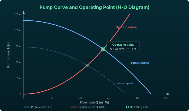
Pump characteristic curves can be created in two ways: parametrically from the design volume flow rate, design head and maximum efficiency — or by polynomial fitting to at least three measured data points (volume flow rate, head, electrical power). The software checks the physical plausibility (efficiency ≤ 1.0) and shows the H-Q curve as a live preview.
Minimum pressure at the pump inlet (NPSH)
Besides the pump head, the pressure on the suction side has to be verified. The governing criterion is the NPSH condition: the NPSH available from the system must exceed the NPSH required by the pump by at least 0.5 m of water column. If that reserve is undercut, the water evaporates inside the suction port and the pump cavitates — even when the absolute pressure at every other point of the network is sufficient.
The available NPSH follows from the absolute pressure at the pump inlet minus the saturation pressure at the operating temperature. The pump inlet is therefore subject to the same lower limit as the high point of the network: saturation pressure plus 0.5 bar against evaporation and cavitation (broad professional consensus) and around 1.0 bar for control tolerance and transients (a planning recommendation), 1.5 bar in total. The derivation and the numbers are given in Meeting Operating Pressure Limits in Heat Networks.
What decides the case is where the pressure maintenance is tied in. With upstream pressure maintenance it sits on the suction side ahead of the pump and sets the inlet pressure directly, so the NPSH condition is usually uncritical. With downstream pressure maintenance the tie-in is on the discharge side, which leaves the suction side one pump head below the imposed pressure level — here the inlet pressure is the critical point and has to be checked separately. Both variants are covered in Pressurization and Expansion.
Index-point control and differential pressure control
Index-point control
Index-point control (differential pressure setpoint control at the index point) is the most efficient control strategy for network pumps. A differential pressure sensor is installed at the hydraulically most unfavourable consumer, and the pump speed is regulated so that the minimum differential pressure the heat transfer station needs for proper operation is always held at that point. It is typically 0.5 to 1.0 bar, with 0.8 to 1.0 bar as the planning value; the technical connection requirements (TAB) of the network operator are binding. The value is derived in Meeting Operating Pressure Limits in Heat Networks.
This method dynamically adapts the pump output to the actual demand and avoids the over-supply of consumers close to the plant.
Constant pressure control
Alternatively, the differential pressure can be kept constant at the pump outlet or another central point. This is simpler to implement but consumes more energy, since the setpoint has to be designed for the maximum case with all consumers at full load. At part load, the excess pressure is then destroyed at the control valves.
Pump models in VICUS Districts:
Four pump models are available: constant-pressure pump, constant-mass-flow pump, controlled pump with a P/PI/PID controller, and a pump with a variable pressure rise. This covers constant-pressure operation, variable-speed operation and index-point control strategies in the dynamic simulation. For index-point control the solver identifies the node with the lowest available differential pressure and adjusts the pump pressure automatically.
Variable speed control and energy savings
Modern network pumps are operated with variable-speed drives that allow stepless speed adjustment. The relationship between speed and power consumption follows the affinity laws:
Reducing the speed to 80 % of nominal lowers the power consumption to , about 51 % of nominal power. Since network pumps run at part load for most of the year, this saves considerable energy compared with unregulated pumps.
Energy demand of network pumps
Typical characteristic values
The pump electricity consumption of a well-designed district heating network is typically 1 to 2 % of the annually transported heat. In poorly dimensioned networks, above all low-temperature networks with small temperature spreads, this share can rise to 5 to 10 % or more.
The electrical pump power is calculated as:
with the total efficiency , the product of hydraulic efficiency, motor efficiency and drive efficiency. For large network pumps, typical total efficiencies lie between 0.60 and 0.75.
Full-load hours approach
To estimate the annual pump electricity consumption, the full-load hours approach is often used:
The part-load factor accounts for the fact that the pump does not run at nominal power on an annual average. Typical values:
| Network type | Operating hours | Part-load factor |
|---|---|---|
| Heating only | 4500 - 5500 h/a | 0.35 - 0.50 |
| Heating + DHW | 6000 - 8000 h/a | 0.30 - 0.45 |
| Cold district heating (year-round) | 7500 - 8760 h/a | 0.25 - 0.40 |
The equivalent full-load hours result from the product and typically lie between 1500 and 3000 h/a.
Practical recommendations
- Minimise pressure losses: generous pipe dimensioning (low specific pressure loss) saves more in pump electricity over the service life than the larger pipes add in investment cost.
- Use index-point control: depending on the network, the energy saving over constant pressure control is 20 to 40 %.
- Provide redundancy: at least two pumps, one running and one on standby, secure the supply during failure or maintenance.
- Use simulation: dynamic network simulation with software such as VICUS Districts computes pressure losses and pump operating points across the whole year.
Getting pump sizing right
Pump sizing is a building block of district heating planning that is often underrated. In conventional networks with a large temperature spread, the effects stay moderate. In low-temperature networks, and cold district heating in particular, an oversized pump system or an unfavourable control strategy can undo the economics of the whole project. The keys to efficient operation with minimum pump electricity are the right pump concept, a careful hydraulic design and variable-speed pumps with index-point control. Tools such as VICUS Districts compute the pump operating points dynamically and report the annual pump electricity consumption as part of the overall balance.
Further reading: Pressure Loss Calculation in District Heating Networks — determining head loss that the pump must overcome, Thermo-Hydraulic Simulation — dynamic analysis of pump operating points over the year, Sizing of Heat Transfer Stations — system integration at the consumer side, Economic Analysis According to VDI 2067 — accounting for pump lifecycle costs in the economic assessment, Pressure Profile and Pressure Diagram — the number behind the minimum differential pressure at the index point, Meeting Operating Pressure Limits in Heat Networks — the minimum pressure at the pump inlet.
References and Standards
- DIN EN 16297 — Pumps — Rotodynamic pumps — Glandless circulators — Requirements and tests
- AGFW FW 524 — Hydraulic Calculation of Hot Water District Heating Networks
- Europump & Hydraulic Institute (2004): Variable Speed Pumping — A Guide to Successful Applications. Elsevier.
Frequently Asked Questions
How is a district heating network pump sized?
What is index-point control for network pumps?
What is the typical pump electricity consumption of a district heating network?
Related Articles
How to size house transfer stations: domestic hot water priority, space heating loads and diversity factors — with sizing guidance for district heating connections.
What is a heating curve and how does it affect the design of district heating networks and heat pumps?
Pump switching and control in district heating networks: parallel and series configurations, redundancy concepts and differential-pressure control.
Basic hydraulic circuits with diagrams: throttle, diverting, mixing and injection circuits for heating, ventilation and district heating compared.
Disclaimer: The content of this page is for general information purposes only and does not constitute legal, planning or engineering advice. All information is provided without guarantee. Despite careful research, VICUS Software GmbH assumes no liability for the accuracy, completeness or timeliness of the information provided. Third-party product names and trademarks are mentioned for informational purposes only and are the property of their respective owners.