Heating Curves — Fundamentals and Application

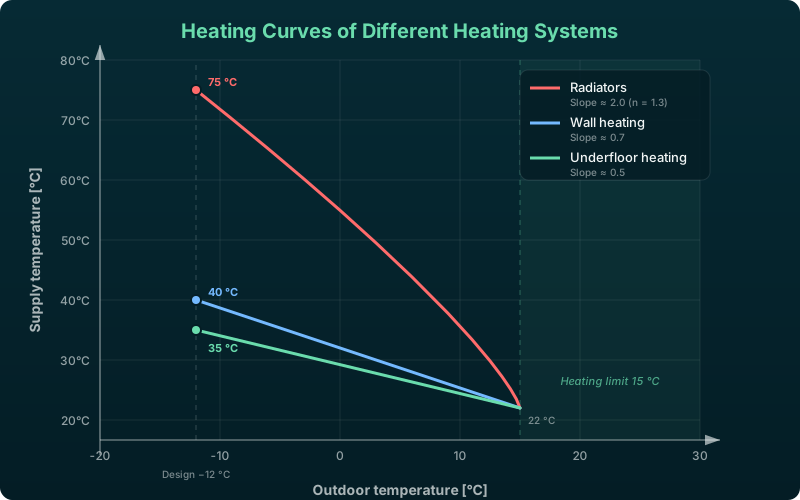
The heating curve describes the relationship between the outdoor temperature and the required supply temperature of a heating system — as the outdoor temperature drops, the supply temperature rises to maintain the desired room temperature. Typical design supply temperatures range from 30—35 °C for underfloor heating to 70—75 °C for conventional radiators, with every Kelvin of lower supply temperature improving the heat pump COP by approximately 2—3 %. The heating curve thereby directly influences the efficiency of heat pumps, the network supply temperature and the achievable seasonal performance factors.

What is a heating curve?

A heating curve (also known as a supply temperature characteristic) defines which supply temperature $T_{\text{VL}}$ the heating system must provide at a given outdoor temperature $T_{\text{a}}$ in order to achieve the desired room temperature $T_{\text{Room}}$. As the outdoor temperature drops, the building’s heat demand increases, and the supply temperature must be raised accordingly.

The simplest relationship is linear:

$T_{\text{VL}} = T_{\text{VL,min}} + s \cdot (T_{\text{a,design}} - T_{\text{a}})$

with the slope (also called gradient) $s$ of the heating curve, the minimum supply temperature $T_{\text{VL,min}}$ (at the heating limit temperature) and the design outdoor temperature $T_{\text{a,design}}$.

The slope follows from the design boundary conditions:

$s = \frac{T_{\text{VL,design}} - T_{\text{VL,min}}}{T_{\text{a,design}} - T_{\text{a,heating limit}}}$

Example calculation

For an underfloor heating system with the following design data:

• Design outdoor temperature: $T_{\text{a,design}} = -12$ °C
• Design supply temperature: $T_{\text{VL,design}} = 35$ °C
• Heating limit temperature: $T_{\text{a,heating limit}} = 15$ °C
• Supply temperature at the heating limit: $T_{\text{VL,min}} = 22$ °C

the slope becomes:

$s = \frac{35 - 22}{(-12) - 15} = \frac{13}{-27} \approx -0{,}48 \; \text{K/K}$

At an outdoor temperature of 0 °C, the supply temperature is:

$T_{\text{VL}}(0\;°\text{C}) = 22 + 0{,}48 \cdot (15 - 0) = 22 + 7{,}2 = 29{,}2 \; °\text{C}$

In practice, heating curves are not always modelled as strictly linear. For radiators in particular, a slightly exponential shape is often used, which accounts for the non-linear heat transfer behaviour of the radiators.

Typical heating curves in comparison

The following table shows typical design supply temperatures and the resulting heating curve slopes for various heat emission systems (at a design outdoor temperature of -12 °C):

The difference is considerable: while underfloor heating requires only 35 °C supply temperature even on the coldest day, a radiator in an older building requires 75 °C. This has direct consequences for the choice of heat generation and for network sizing.

Influence on the COP of heat pumps

The Coefficient of Performance (COP) of a heat pump depends decisively on the temperature difference between the heat source and the heat sink. The theoretical Carnot COP is:

$\text{COP}_{\text{Carnot}} = \frac{T_{\text{VL}}}{T_{\text{VL}} - T_{\text{source}}}$

where the temperatures must be entered in Kelvin. In practice, heat pumps achieve about 40 to 55 % of the Carnot COP (quality grade).

For a source temperature of 0 °C (273 K) and various supply temperatures, a quality grade of 0.50 yields:

Every Kelvin of lower supply temperature improves the COP by approximately 2 to 3 %. An underfloor heating system with a 35 °C supply temperature therefore achieves a COP that is roughly 75 % higher than that of a conventional radiator operating at 70 °C — an enormous difference in the annual energy balance.

Heating curve and district heating network planning

Network supply temperature

The heating curve of the most critical consumer (i.e. the one with the highest supply temperature requirement) determines the required network supply temperature. In a network with mixed consumer types — new buildings with underfloor heating and existing buildings with radiators — the network supply temperature must meet the requirements of all consumers plus the approach temperature of the transfer stations:

$T_{\text{VL,network}}(T_a) = \max_i \left[ T_{\text{VL},i}(T_a) \right] + \Delta T_{\text{approach}}$

This means that a single consumer with a high supply temperature requirement can raise the entire network temperature level. In practice, it is therefore assessed whether local reheating (for example via a decentralised heat pump) is more economical for such consumers than a general increase of the network temperature.

Gliding network operation

In modern district heating networks, the network supply temperature is operated in dependence on the outdoor temperature (gliding operation). At mild temperatures, the network supply temperature drops, which significantly reduces the heat losses. The network heating curve forms the envelope of all consumer heating curves:

• In winter at -12 °C: network supply temperature e.g. 75 °C
• In the transition period at 5 °C: network supply temperature e.g. 55 °C
• In summer (DHW only): network supply temperature e.g. 60 to 65 °C

The summer reduction is limited in networks that only have to provide domestic hot water, since the supply temperature for DHW preparation must be at least 58 to 65 °C.

Application in cold district heating networks

In cold district heating networks, the network heating curve in the classical sense no longer applies, since the network is operated at a low, almost constant temperature level. The heating curve is fully shifted to the building-side heat pump, which raises the temperature level individually. This has the advantage that each building generates its optimum supply temperature independently of the others — without compromises due to differing consumer requirements.

Optimising the heating curve

A heating curve that is too steep leads to unnecessarily high supply temperatures and thus to:

• Higher network losses
• Lower heat pump COP
• Higher energy consumption

A heating curve that is too flat causes the rooms to be insufficiently heated at low outdoor temperatures. The optimum setting requires a careful tuning to the building, the heat emission surfaces and the user behaviour. In practice, fine-tuning is often carried out during the first year of operation through monitoring and readjustment.

Recommended approach:

1. Perform a heat load calculation according to DIN EN 12831
2. Dimension the heat emission surfaces and derive the design supply temperature from them
3. Calculate the heating curve and store it in the control system
4. Adjust the parallel shift if necessary (vertical shift of the curve by 2 to 3 K in case of systematic under- or over-supply)

Conclusion

The heating curve is much more than a simple control curve — it is a central planning parameter that influences the efficiency of the entire heat supply system. Low supply temperatures, made possible by surface heating systems and well-insulated buildings, are the key to high heat pump performance factors and low network losses. When planning district heating networks, the heating curve of every connected building should be known, since it decisively determines the network supply temperature and thus the network losses. VICUS Districts takes into account the heating curves of all consumers in the network design, while VICUS Buildings can derive the building-side heating curve from the dynamic building simulation. In cold district heating networks, this problem is elegantly circumvented since the decentralised heat pumps supply each building individually.

Further reading: Sizing of Heat Transfer Stations — station control and the role of the heating curve, Network Temperatures in District Heating Networks — how supply temperature design shapes the entire network, Low-Temperature District Heating: Fundamentals — low-temperature operation where building-side heating curves become critical, Dynamic Building Simulation — using simulation to predict heating loads and derive optimal curves.

References and Standards

• DIN EN 12831 — Energy performance of buildings — Method for calculation of the design heat load
• VDI 6030 Part 1 — Designing room heating systems — Fundamentals and design of room heating systems
• DIN EN 12828 — Heating systems in buildings — Design for water-based heating systems