Simulation with multiple energy plants

District heating network, part 9: thermo-hydraulic simulation with multiple feed-in points

Overview ▶ 0:09

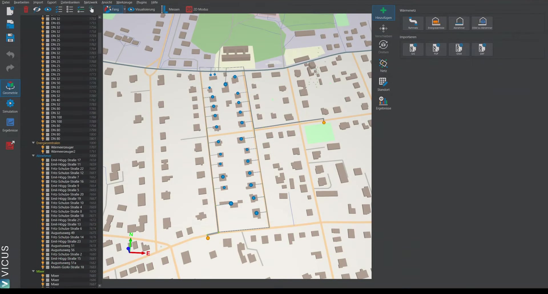
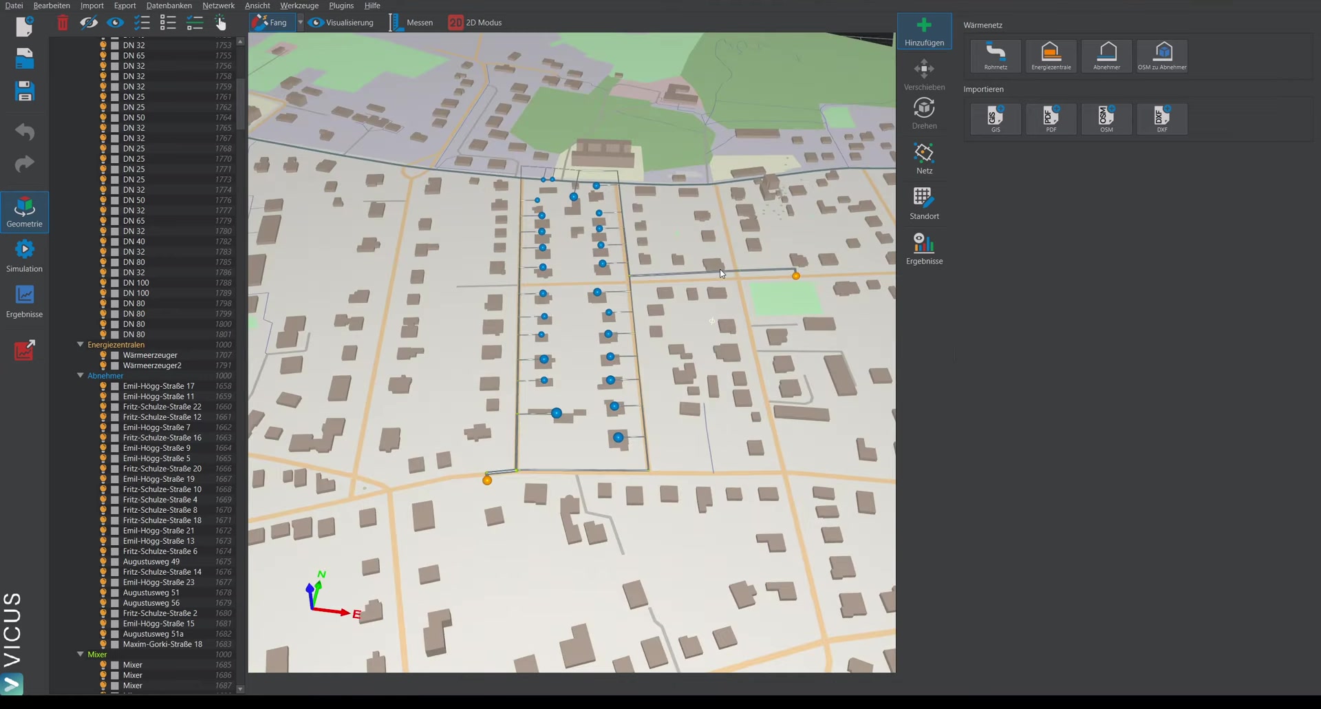
District heating network with two energy plants ready for simulation — Starting point: network with two energy plants after completed pipe sizing

This tutorial demonstrates how to perform a steady-state simulation with multiple energy plants. The starting point is the network from the previous video, in which the pipe sizing with two energy plants has already been performed.

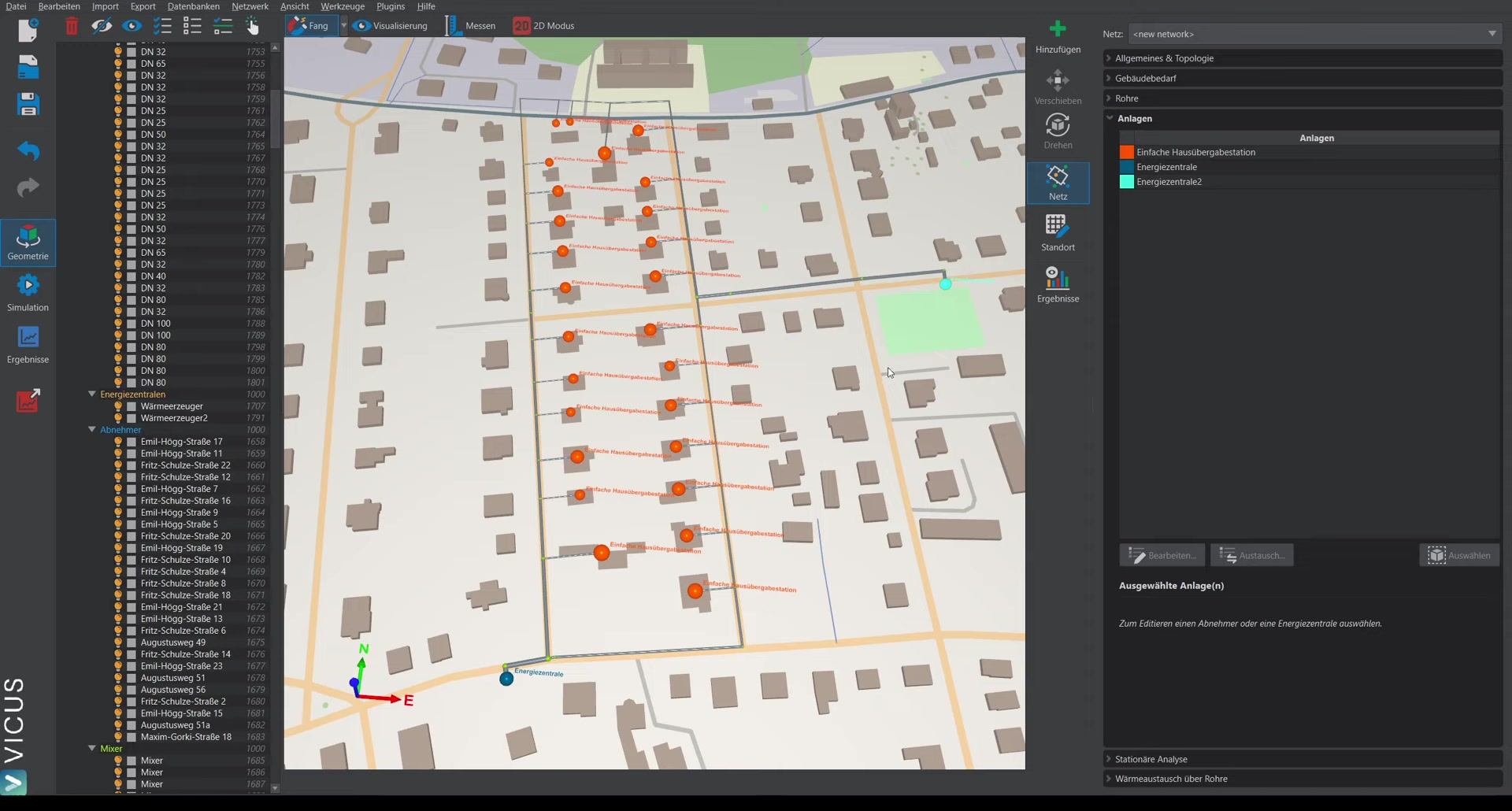
Assigning a system to the second energy plant ▶ 0:36

Assignment of a system with a different head to the second energy plant — Assignment of a copied system with a different head (1.0 bar) to the second energy plant

The newly created energy plant does not yet have a system assigned. The procedure is:

Assign a new system from the database — copy the existing energy plant.
Assign a name, e.g. “Energy plant 2”.
In the editor, set a different head (e.g. 1.0 bar) to study the effect on the heat feed-in.

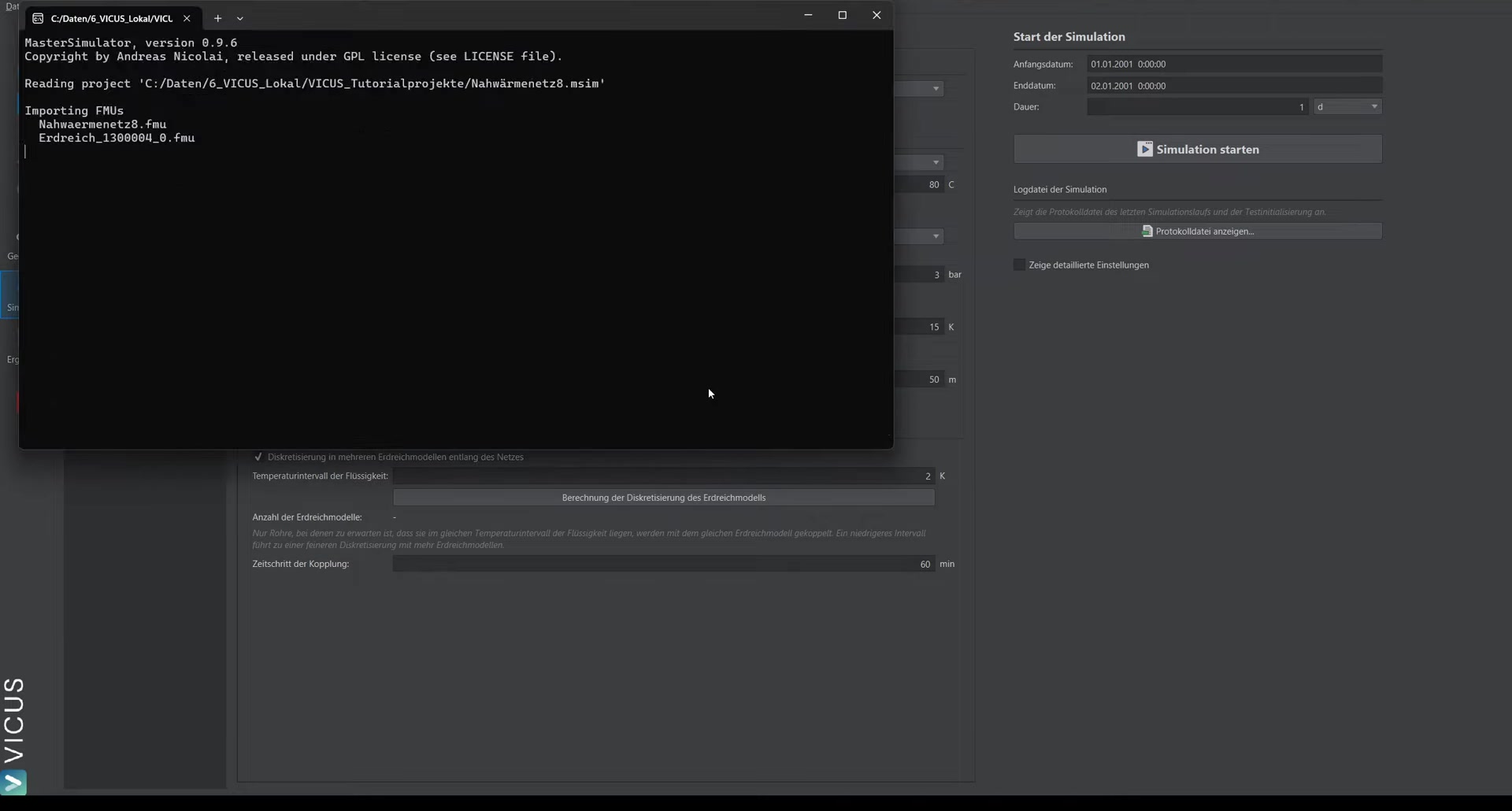
Steady-state simulation with constant demand ▶ 1:58

Dynamic simulation with constant demand over one day as steady-state substitute — Dynamic simulation with constant demand over one day — quickly establishes a steady state

The steady-state analysis in this version only works with a single energy plant. Instead, the dynamic simulation is used with a constant demand at the consumers:

Switch to Building demand.
Using smart selection, select all consumer nodes.
In the demand model, set a constant demand.
Start the simulation over one day — with constant values, a steady state is quickly reached.

Evaluating the results ▶ 3:44

Fed-in heating power of both energy plants: 369 kW and 165 kW — Results: heat generator 1 feeds in approx. 369 kW, heat generator 2 (1.0 bar) approx. 165 kW

After the simulation, the results under Energy plant show the heating power fed in by each energy plant:

Heat generator 1: approx. 369 kW
Heat generator 2 (with 1.0 bar head): approx. 165 kW

Checking the temperature difference ▶ 4:32

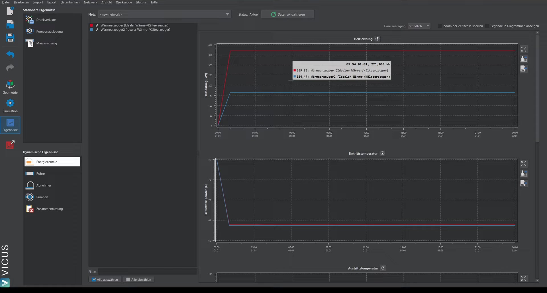
Check of the 15 K temperature difference at the consumers — Check: 15 K temperature difference at the consumers — a clear deviation indicates undersized pumps

Important: Even in steady-state simulations, you must check whether the desired temperature difference (here 15 Kelvin) is reached at the consumers. If the temperature difference rises significantly, this is a sign that the pumps are undersized.

Investigating the effect of the pump pressures ▶ 5:19

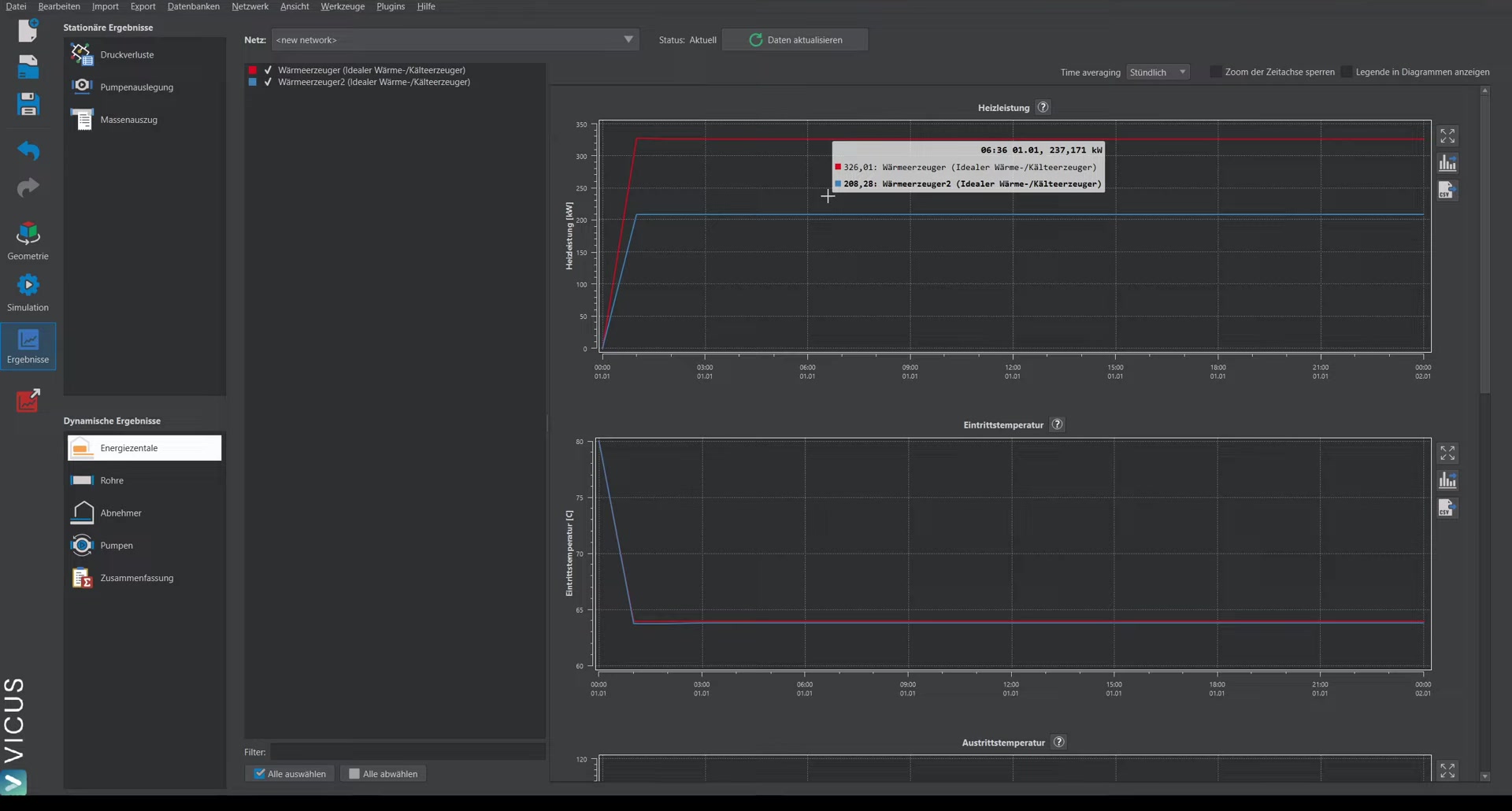
Changed heat feed-in after increasing the head to 1.5 bar — Effect of the head: heat generator 2 with 1.5 bar feeds in 200 kW, heat generator 1 drops to 326 kW

By changing the pump head, the effect on the heat feed-in can be investigated iteratively:

Increase the head of the second energy plant to, for example, 1.5 bar.
Start the simulation again.
The results show: heat generator 2 now feeds in approximately 200 kW (previously 165 kW), while heat generator 1 has dropped from around 400 kW to 326 kW.

Transition to dynamic simulation ▶ 6:28

Switching from constant demand to predefined time series for annual simulation — Transition to annual simulation: switch the demand model from constant demand to a predefined time series

With this method, you can iteratively check which heat generator feeds in how much heat — initially for the peak load case. For a dynamic annual simulation, the demand model is simply switched back to a predefined time series:

Select all consumers.
Instead of constant demand, select Predefined time series again.
The annual simulation can then be carried out as usual.