Configure heating curve & limit outlet temperature

District heating network, part 5: configure the heating curve and limit the outlet temperature of the transfer stations

Overview ▶ 0:09

District heating network for configuring a heating curve and outlet temperature limit — Configuring a heating curve to limit the outlet temperature and represent undersupply situations

This tutorial demonstrates how to represent undersupply in a simplified way and limit the outlet temperature of the transfer station by configuring a heating curve.

The simple heat-exchanger model ▶ 0:31

Simple heat-exchanger model without considering the supply temperature — Simple model: heat extraction according to the building's demand, without taking the inlet temperature into account

With the simple house transfer station using the simple heat exchanger, heat is always extracted from the network according to the configured building demand. Initially, this model does not consider which supply (i.e. inlet) temperature is actually available from the network. This can lead to heat being extracted during start-up conditions — when the network has cooled down — even though the inlet temperature is not sufficient.

Activating the outlet temperature limit ▶ 1:25

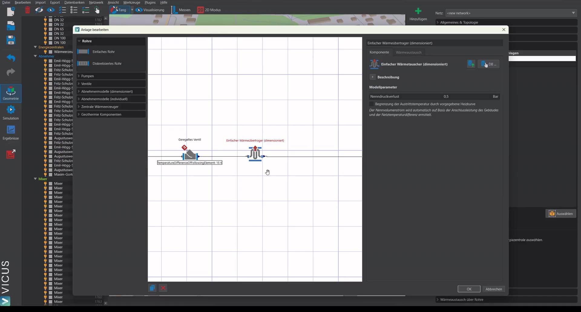
Activating the outlet temperature limit via heating curve in the system — Activating the option to limit the outlet temperature via the specified heating curve

To account for this effect, there is the option Limit outlet temperature via the specified heating curve. It is activated in the house transfer station’s system.

Configuring the heating curve ▶ 1:39

Configuration of the heating curve with 70 °C supply temperature and 15 K spread — Configuring the heating curve: constant supply temperature 70 °C on the secondary side with 15 K temperature difference

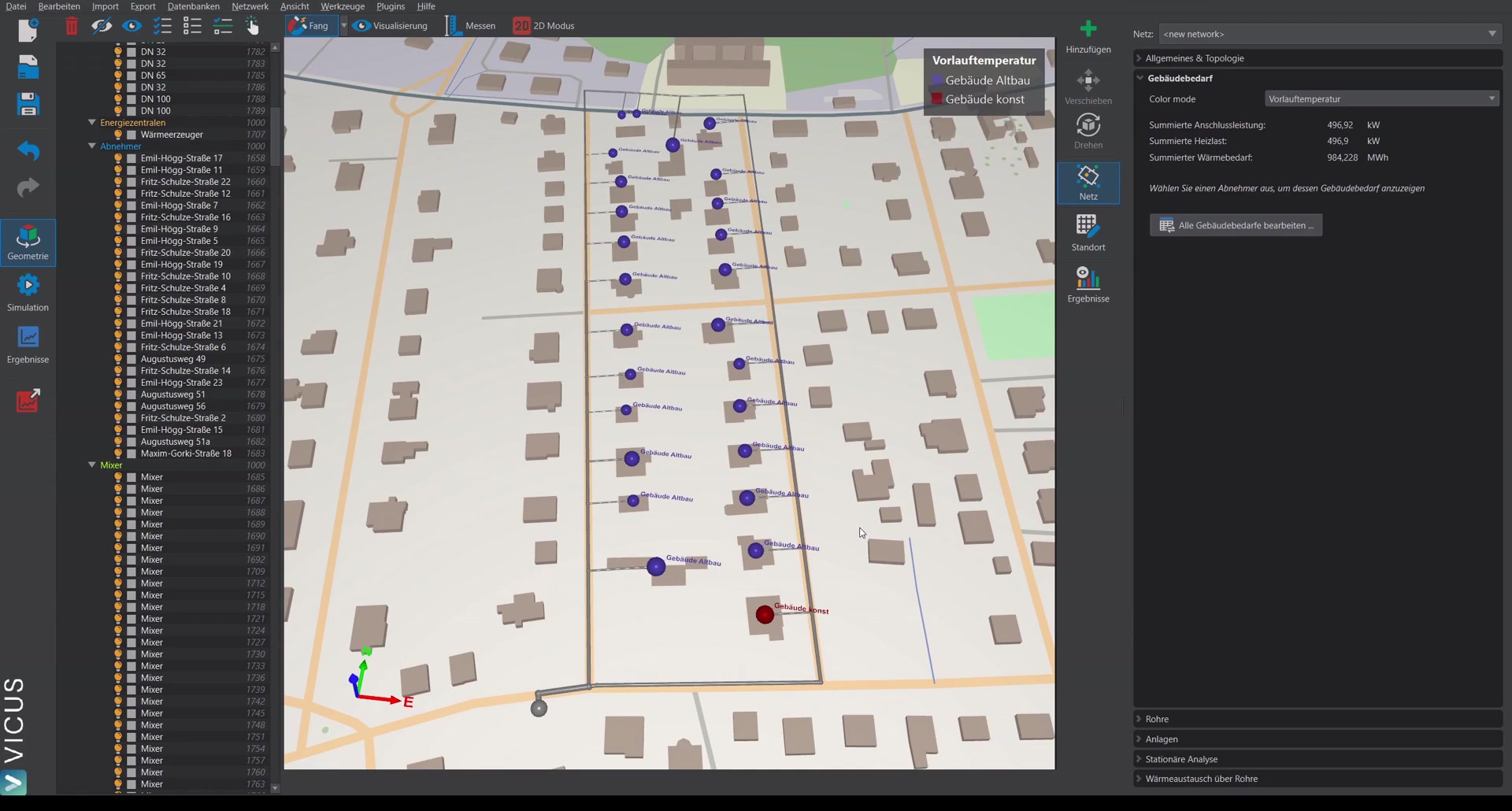
The heating curve is configured via Building demand:

Select a consumer.
Edit the Supply temperature of the heating option.
The preset heating curve is a database element. To make changes, create a copy.
For this example, a constant function is set: the secondary-side supply temperature is 70 °C with a 15 Kelvin temperature difference.
Assign a meaningful name (e.g. “Building constant”) and select it.

Note: The specified supply temperature refers to the secondary side, i.e. the building, not to the network.

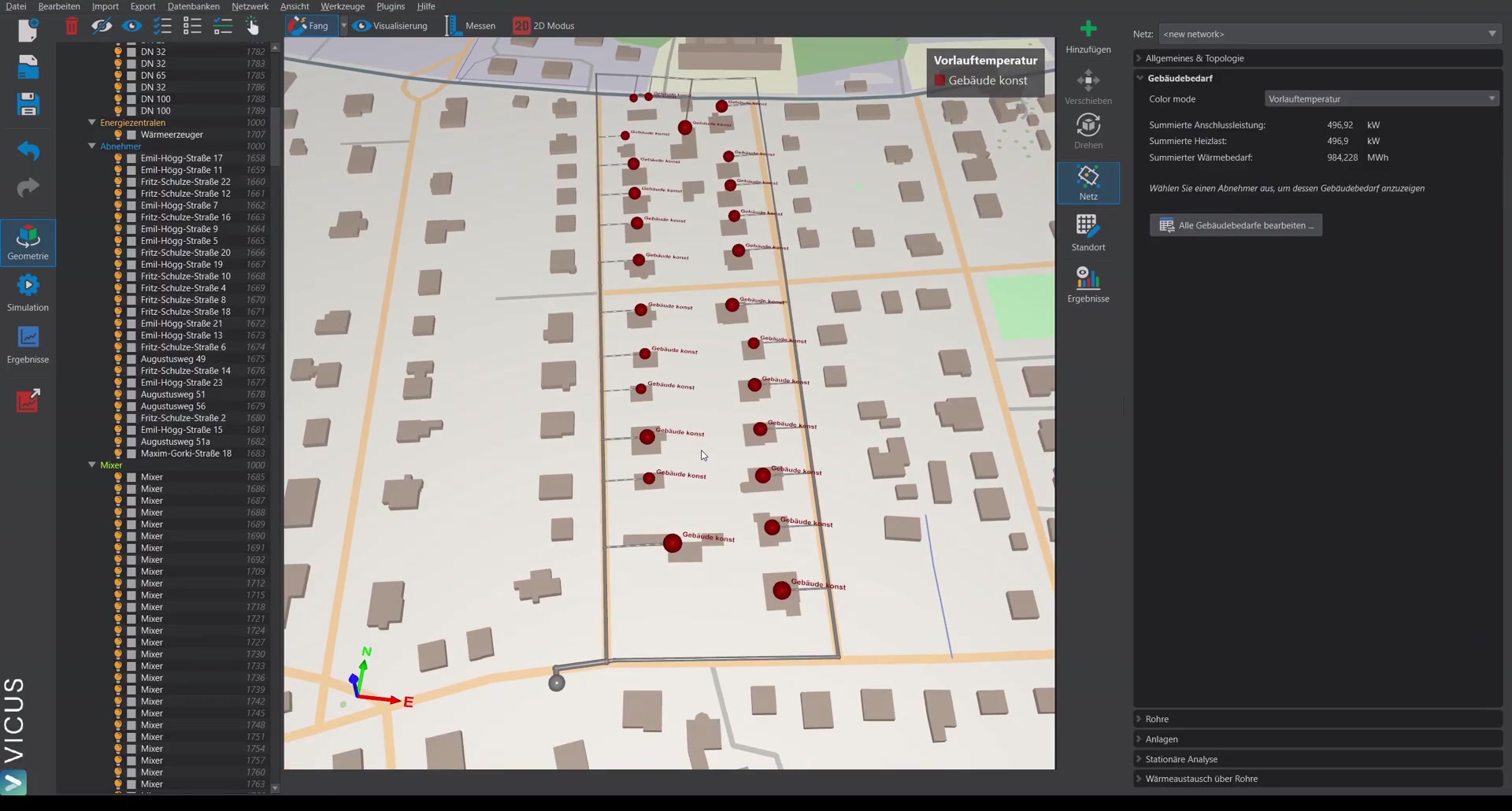
Assigning the heating curve to all buildings ▶ 3:41

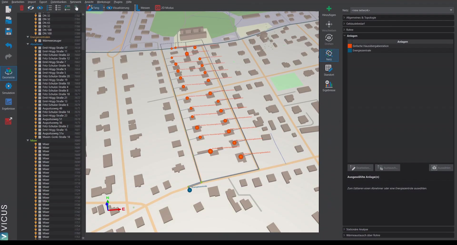
Assignment of the heating curve to all buildings via smart selection — Simultaneous assignment of the heating curve to all consumers via Ctrl key or smart selection

To assign the heating curve to all buildings at the same time, there are two options:

Use the Ctrl key and a selection window to select the entire network and change the heating curve.
Via smart selection, select all consumers directly — here you can additionally filter by connection load or name.

Simulation with heating curve ▶ 4:47

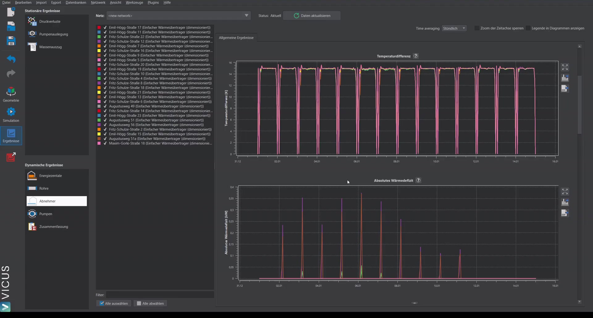
Simulation results with small heat-deficit peaks during network start-up — Results: small heat-deficit peaks during network start-up conditions (uncritical at 0.3-0.4 kW)

After starting the simulation with the activated outlet temperature limit, the results show:

The spread on the primary side remains at 15 Kelvin.
Under Absolute heat deficit, small peaks appear. The heat deficit indicates the amount by which the current heating power falls short of the building’s heat demand. The peaks occur at moments when the network is just restarting and there is briefly a small undersupply. In this case the values are low (about 0.3 to 0.4 kW) and can be classified as uncritical.

Lowering the supply temperature in the network ▶ 6:37

Clear heat deficit with lowered supply temperature of 70 °C — Lowered network supply (70 °C): clear heat deficit with persistent undersupply of 2-3 kW

Under Databases > Heating curves, both the building heating curve and the network supply temperature can be inspected. If the supply temperature in the network is lowered from 80 °C to 70 °C, the picture changes significantly:

On the primary side, the temperature difference remains at about 15 Kelvin.
The heat deficit is now clearly visible — no longer just small peaks, but a persistent undersupply of up to 2 to 3 kW at some consumers.

This shows that the supply temperature in the network cannot be lowered arbitrarily without compromising security of supply.