Thermo-hydraulic simulation

District heating network, part 3: run a dynamic thermo-hydraulic simulation and evaluate the results

Overview ▶ 0:08

District heating network ready for dynamic thermo-hydraulic simulation — Starting point: the parameterized network for dynamic thermo-hydraulic simulation

This tutorial demonstrates how to simulate the network dynamically and evaluate the results. In the previous videos, the network was already created and the steady-state calculation was performed.

Ground boundary conditions ▶ 0:27

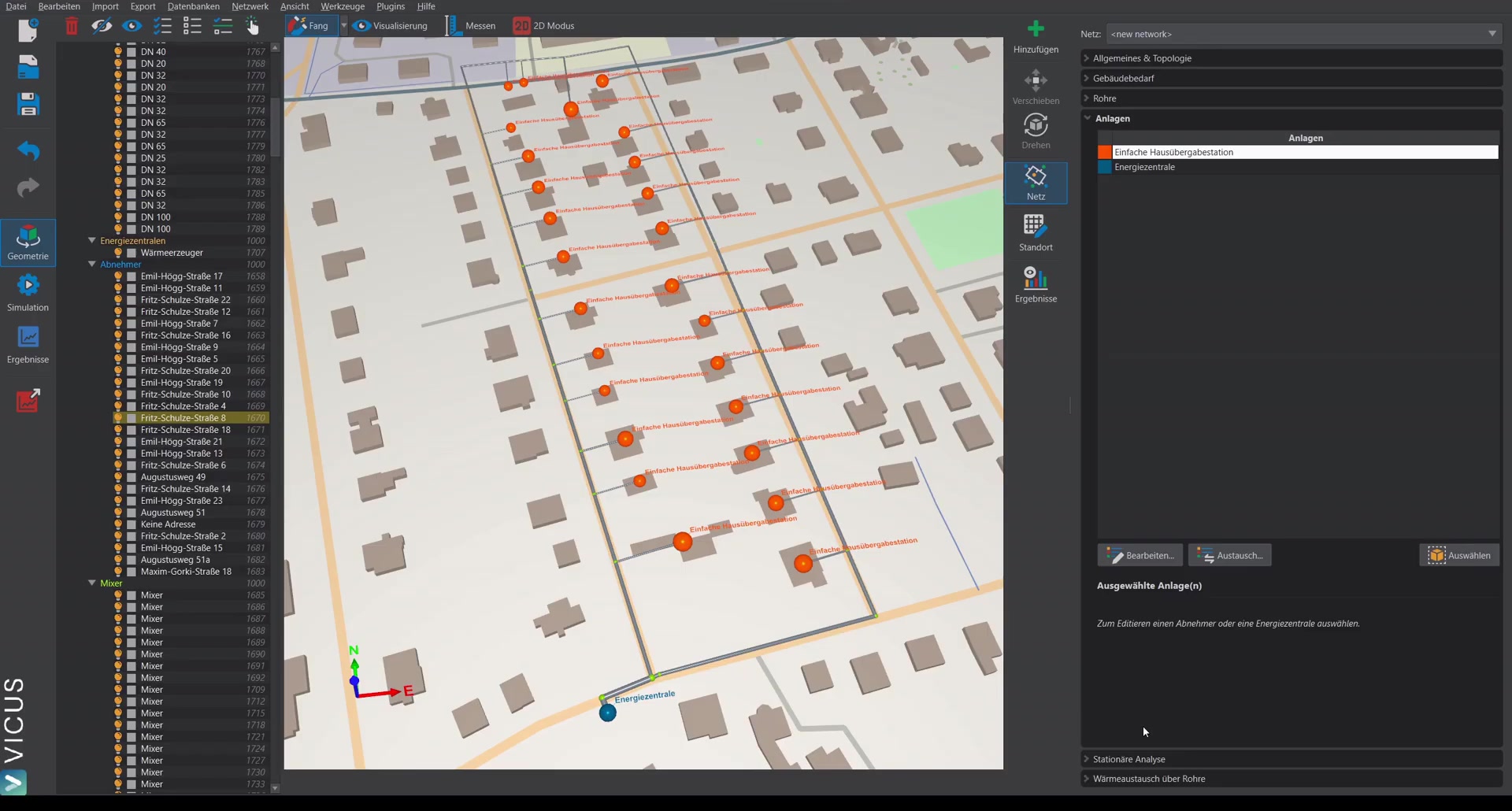
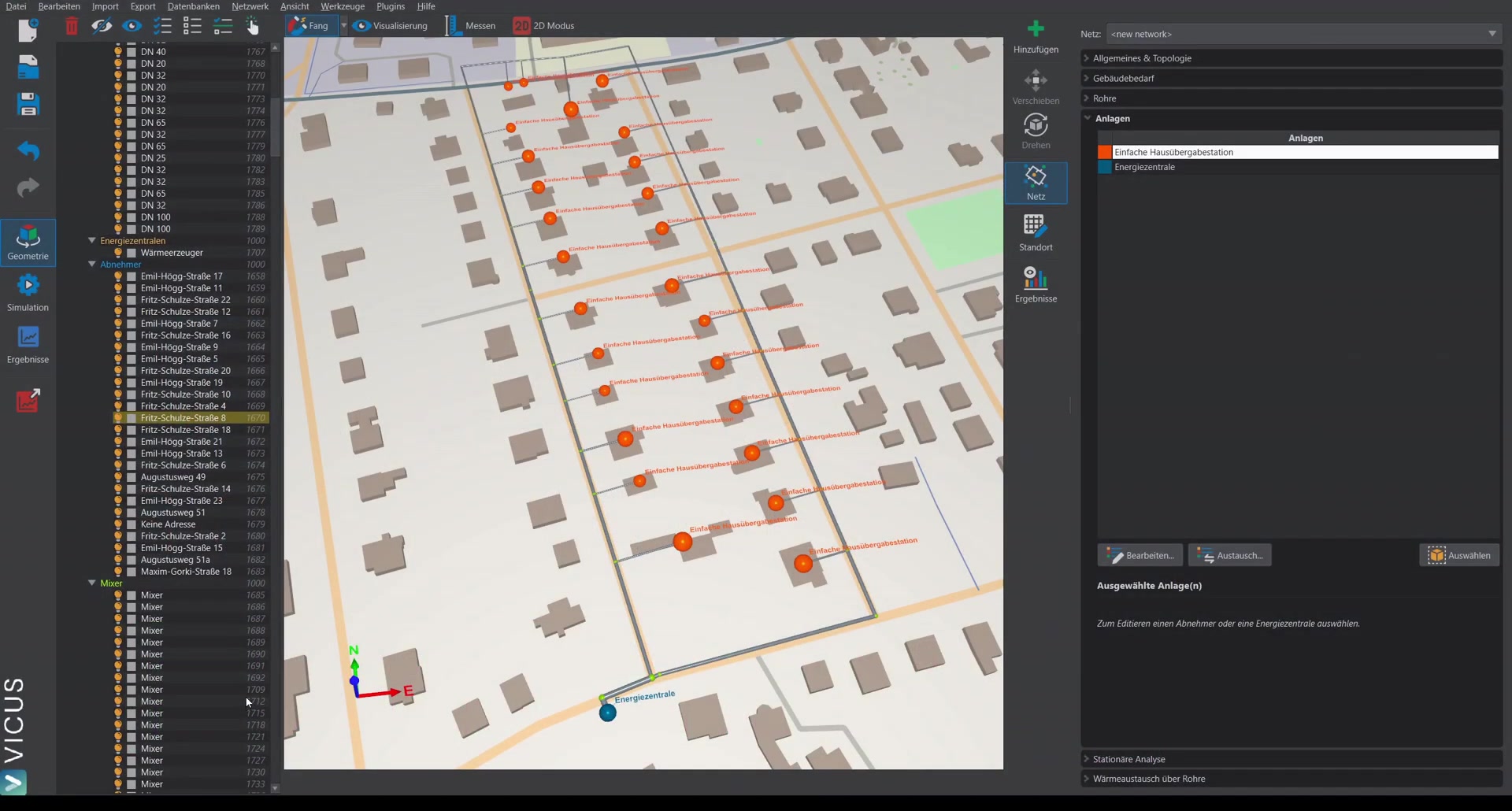
Ground boundary conditions with soil type, burial depth, and moisture content — Configuration of the ground boundary conditions: soil type, burial depth, pipe spacing, and moisture content

On the right side, the final network property you can configure is the boundary conditions for the ground and the pipe network. By default, a ground model is already assigned as the boundary condition. Alternatives are:

A constant temperature
A time-dependent temperature
The full ground model (most detailed option)

With the ground model, you can additionally specify the soil type, the burial depth of the pipes, the pipe spacing, and the moisture content.

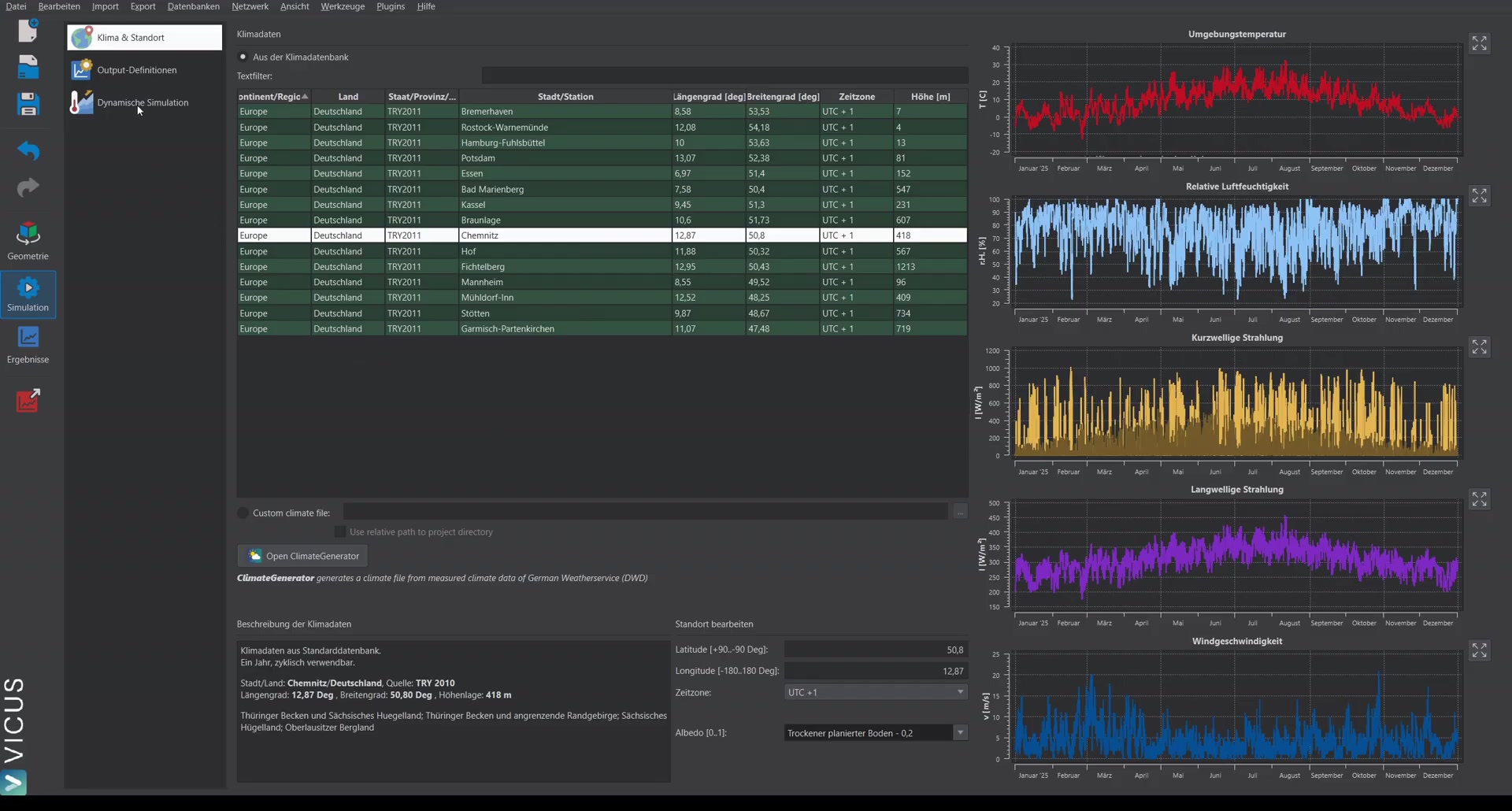
Selecting climate data ▶ 1:21

Selection of climate data from test reference years of the German Weather Service — Selection of climate data: pre-installed test reference years or your own data in DAT/EPW format

On the simulation page, the climate is selected first. Several test reference years of the German Weather Service are pre-installed. Custom climate data can be imported in the German Weather Service’s DAT format or in EnergyPlus’s EPW format.

Starting the simulation ▶ 2:02

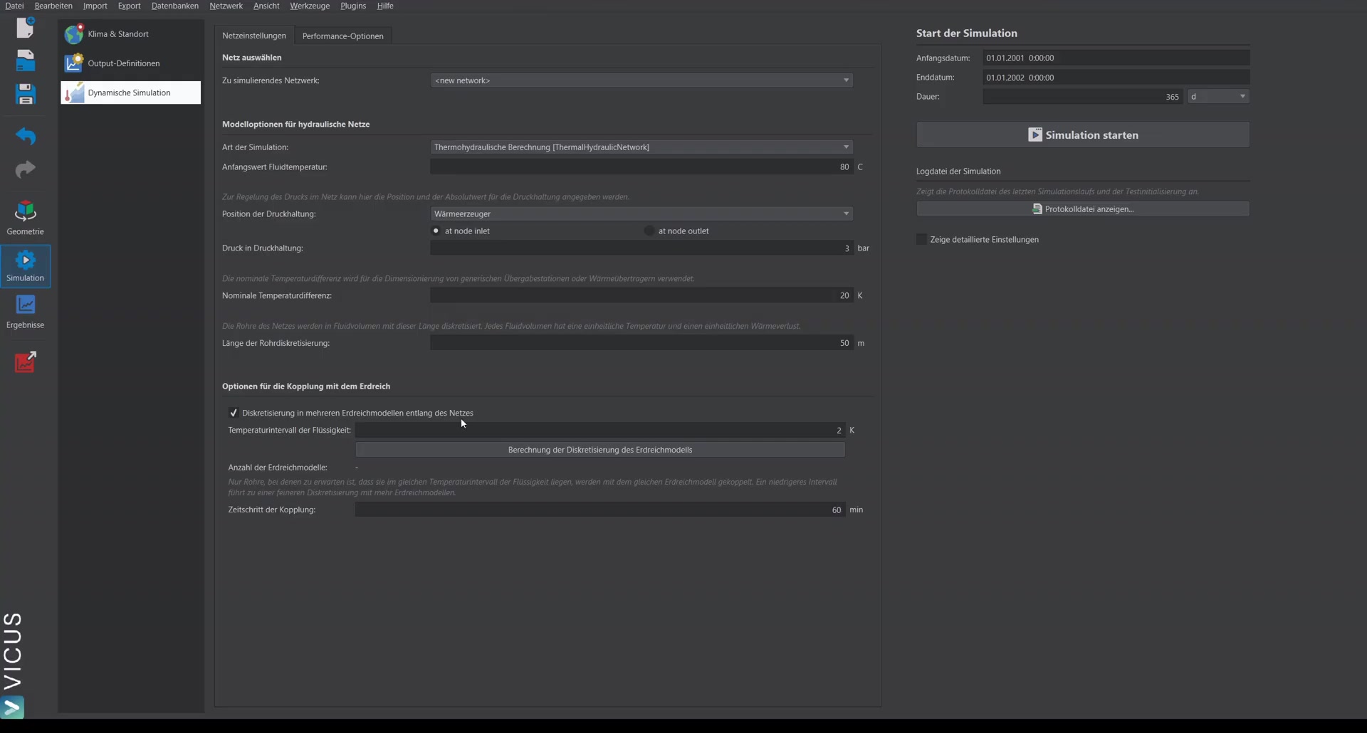
Simulation settings with static pressure and start as separate process — Starting the dynamic simulation as a separate background process with default settings

Click Dynamic simulation.
Check the simulation settings — the defaults are usually sufficient. Among other things, the static pressure is specified as a reference pressure at an energy plant.
Start the simulation — it runs as a separate background process and takes about 10 to 12 minutes for this example network.

Evaluating the results ▶ 2:47

Results view with refresh option during the ongoing simulation — Result evaluation: already available during the running simulation via the Refresh button

The results can already be inspected during the running simulation via the results view and the Refresh button.

Energy plant ▶ 3:09

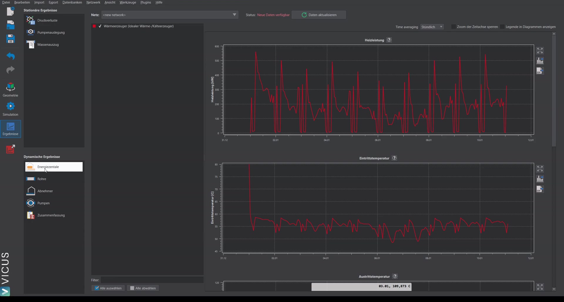
Results of the energy plant with heating power, temperatures, and volume flow — Energy plant: heat output, inlet/outlet temperature, and volume flow over the year

Under Energy plant, the following is shown: heat output (heating power), inlet and outlet temperature, and volume flow.

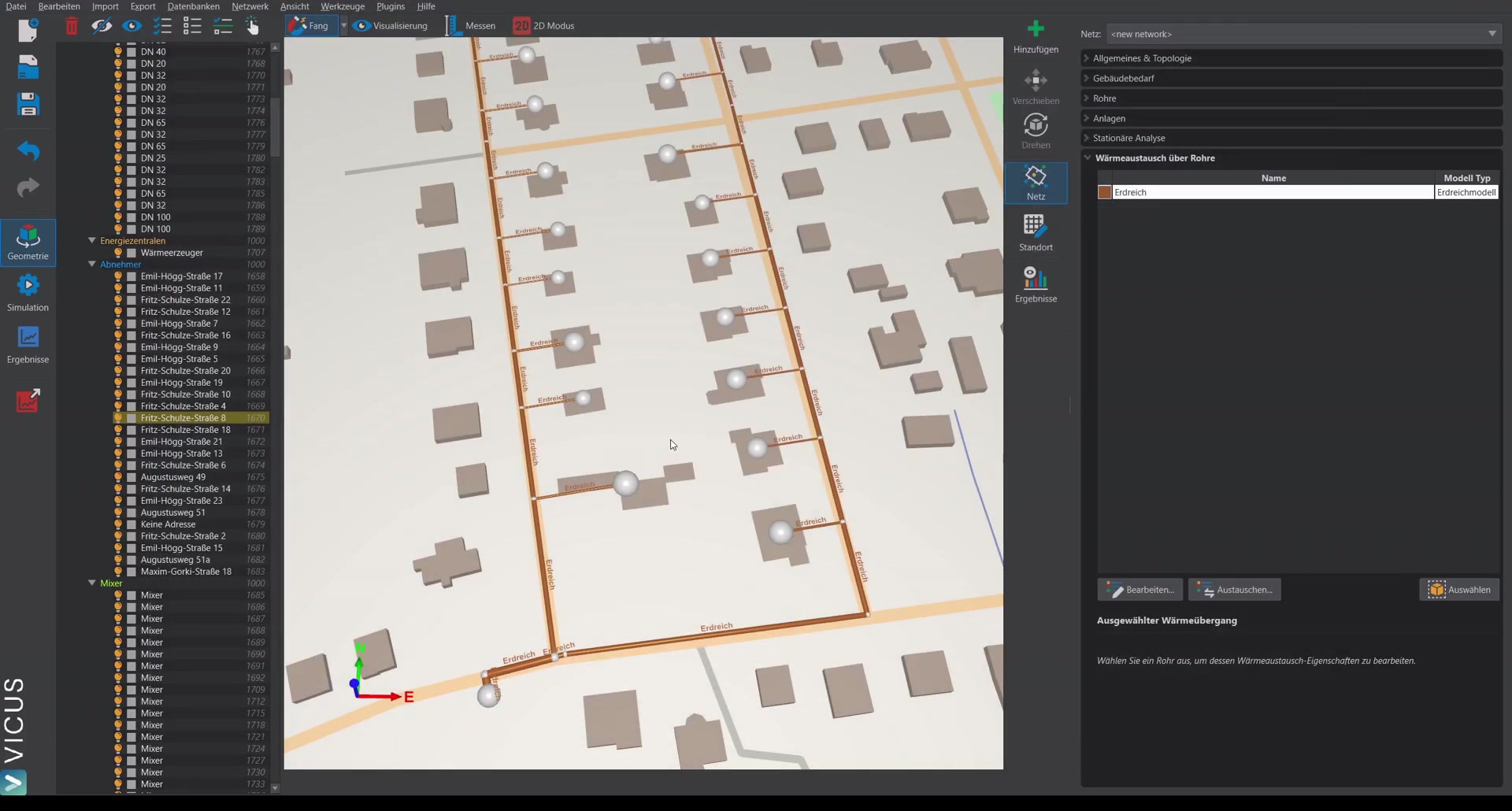
Pipes ▶ 3:21

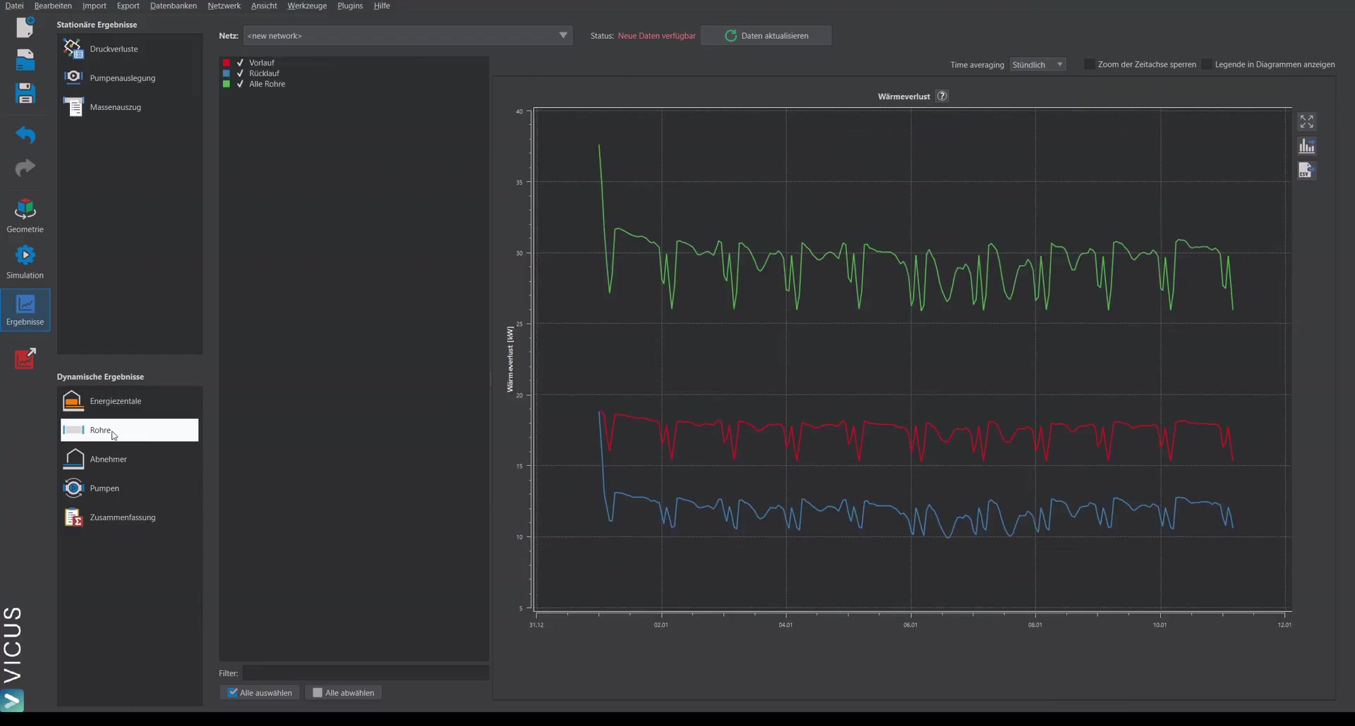
Heat loss of the pipe network split into supply and return — Heat losses: split into supply and return as well as total heat flow to the ground

Under Pipes, the heat loss of the pipe network is shown — split into supply and return, as well as the total heat flow to the ground.

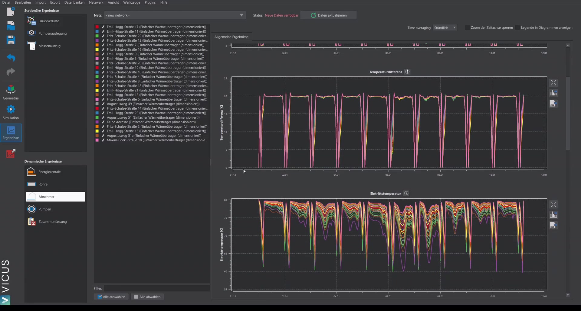
Consumers ▶ 3:35

Consumer results with heating power and temperature difference — Consumers: heating power and temperature difference — critical check on compliance with the 20 K target

Under Consumers, the delivered heating power and the temperature difference are displayed.

Important: In every simulation, the temperature difference should be critically checked. The consumers regulate on a prescribed temperature difference (here 20 Kelvin). If this is exceeded, it may indicate that the pump is undersized or the network is undersized.

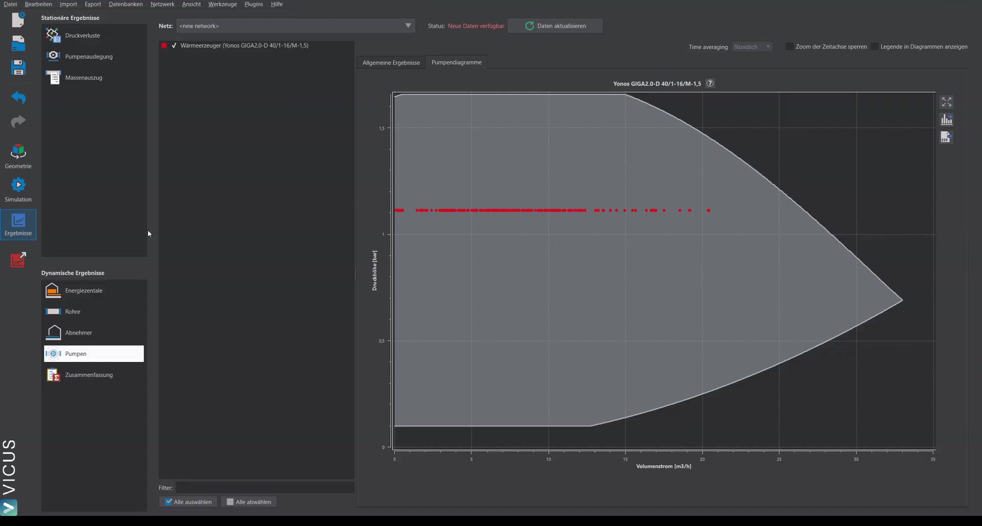
Pump ▶ 4:34

Pump diagram with operating points in the context of the operating range — Pump diagram: running operating points in the context of the pump's operating range

Under Pump, the inlet and outlet temperature, efficiency, and volume flow are displayed. In the separate Pump diagram tab, the running operating points during the simulation can be displayed in the context of the pump’s operating range — this lets you check whether the pump is adequately sized.

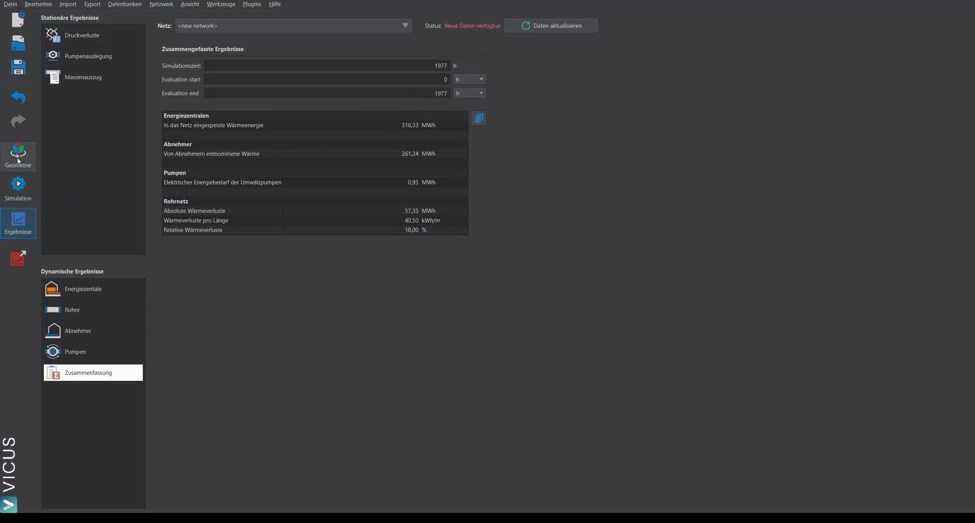
Summary ▶ 5:19

Summary with supplied heat, extracted heat, and percentage losses — Summary: supplied and extracted heat as well as percentage network losses

At the bottom there is a summary, where you can evaluate how much heat was supplied to and extracted from the network and how large the losses are. The losses are also shown as a percentage. The simulation has completed when 8760 hours of simulation time are reached.

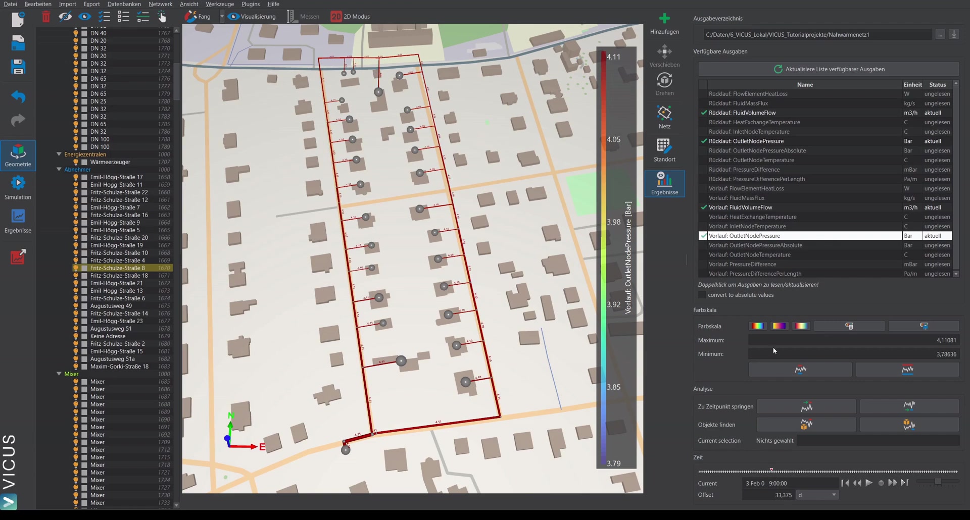
Interactive result display ▶ 5:52

Interactive result display with color scale and time slider on the network plan — Interactive result display: volume flow, pressure, or temperature with time slider directly on the network

In the geometry view, the result view on the right offers another way to display results interactively on the network:

Select the desired result quantity (e.g. volume flow, pressure, temperature).
Navigate through the entire simulation time with the time slider.
Jump to specific points in time via buttons (e.g. to the time of maximum volume flow).
Adjust the color scale either to the current time or to the entire simulation period.

Analyzing temperature distribution ▶ 7:22

Temperature distribution in the network shows sections with little flow — Temperature distribution: quick detection of sections with little or no flow

The temperature distribution makes it easy to spot sections with little or no flow — for example, when one consumer is supplied from one side and another consumer from the other side.