Hydraulic Balancing

Hydraulic balancing ensures that every consumer in a district heating network receives exactly the volume flow rate it needs, with neither over- nor under-supply. Four systems are in use: static balancing with balancing valves, automatic differential pressure controllers, combination valves with a valve authority of 1.0, and electronic pressure-independent valves with ultrasonic flow measurement. Without correct balancing, return temperatures rise and pump energy consumption climbs, and even a perfectly sized pump cannot guarantee uniform supply.

Static Hydraulic Balancing

In static hydraulic balancing, each consumer is assigned a control valve that regulates the volume flow rate according to the current heat demand. In addition, a balancing valve limits the maximum volume flow rate in its branch through a fixed presetting. The aim is to deliver exactly the design volume flow rate at every consumer under full load.

The balancing valve is set to a fixed resistance during commissioning. It throttles the differential pressure in the respective branch so that no consumer is over- or under-supplied under design conditions. The setting values are derived from the pressure loss calculation of the network.

Problems During Part-Load Operation

Static balancing only works reliably under design conditions. As soon as individual consumers go into part load and their control valves close, the pressure distribution in the network shifts. The available differential pressure at the remaining open consumers rises, and balancing valves with fixed presettings cannot compensate for that increase. Consumers in full-load branches are then over-supplied, so return temperatures rise and network efficiency drops, while consumers in hydraulically unfavourable branches may still be under-supplied.

A constant pump control curve, meaning a fixed differential pressure at the pump, makes this worse. When the total volume flow rate falls during part load, the available differential pressure in the network rises even further. Flow rates at the consumers with open valves increase, which brings excessively high return temperatures (the volume flow rate exceeds what heat transfer needs), higher pump power consumption and noise at heavily throttled valves.

Static balancing is therefore only conditionally suitable for small networks with few consumers and limited part-load variation.

Automatic Differential Pressure Controller

The automatic differential pressure controller solves the central problem of static balancing. It keeps the differential pressure across a system section, such as a branch or a transfer station, constant regardless of the load in the rest of the network. The setpoint typically lies between 10 and 100 kPa and is set during commissioning.

Operating Principle

The controller is a self-acting valve with a spring-loaded diaphragm. It senses the differential pressure across the protected section through impulse lines. If the differential pressure rises above the setpoint, for example because neighbouring consumers go into part load, the controller closes and throttles the excess. If it falls below the setpoint, the controller opens accordingly.

Advantages

The differential pressure at the control valve stays constant regardless of the load in other branches, so there is no over- or under-supply. The valve always works under defined pressure conditions, which keeps control behaviour stable and free of oscillation. And because every branch receives its intended differential pressure, return temperatures and heat transfer remain in the optimal range independently of the balancing state.

Pump Control Curve

With automatic differential pressure controllers, a proportional pump control curve is recommended: the pump’s differential pressure setpoint decreases as the volume flow rate decreases. This cuts pump power consumption during part-load operation. The minimum delivery pressure must be chosen so that, even at part load, enough differential pressure remains at the hydraulically most unfavourable consumer for the differential pressure controller and the control valve to work properly.

Limitations

When using automatic differential pressure controllers, the minimum valve authority of the downstream control valves must be maintained. The valve authority $P_V$ describes the ratio of the pressure drop across the control valve to the total pressure drop of the controlled circuit:

$P_V = \frac{\Delta p_{\text{valve}}}{\Delta p_{\text{valve}} + \Delta p_{\text{circuit}}}$

For good control quality, $P_V \geq 0.5$ should be achieved. If the valve authority is too low, the control valve reacts disproportionately to small stroke changes, which can lead to unstable control behaviour.

Combination Valve (Pressure-Independent Control Valve)

The combination valve unites a differential pressure controller and a control valve in a single housing. The pressure differential across the control valve section is factory-set to a fixed value, typically 20 kPa. The integrated differential pressure controller compensates changes in network pressure without affecting the valve’s control characteristic.

Valve Authority

The decisive advantage of the combination valve is its valve authority of $P_V = 1.0$. Since the differential pressure controller absorbs all external pressure changes, the entire usable differential pressure always drops across the control valve section, and the variable pressure drop across the controlled section no longer matters for the control function. The valve therefore keeps optimal control characteristics under every operating condition.

Advantages

The combination valve retains all advantages of the automatic differential pressure controller. Mass flow rate changes in one branch do not affect the control quality of neighbouring branches, because each valve regulates its own differential pressure. Planning is simpler, since valve authority and differential pressure are factory-defined, and the single housing is more compact than a separate differential pressure controller plus control valve.

Pump Control Curve

As with the separate differential pressure controller, a proportional pump control curve with minimum delivery pressure is recommended. The minimum delivery pressure must be set so that the input differential pressure required by the combination valve is reliably available at the hydraulically most unfavourable consumer.

Electronic Pressure-Independent Control Valve

Electronic pressure-independent control valves are the most recent development in hydraulic balancing. In place of a mechanical differential pressure controller, they use real-time ultrasonic flow measurement. The current flow rate is measured continuously and compared with the setpoint, and an electronic actuator corrects the valve opening whenever the two diverge.

Operating Principle

The valve receives a flow setpoint from the supervisory controller, for example a building automation system. Its integrated ultrasonic sensor measures the actual flow rate without moving parts and without pressure loss. When the actual value drifts from the setpoint, say because of pressure changes in the network, the actuator adjusts the valve position until the two match again.

Advantages

Because there is no mechanical differential pressure controller with its own pressure loss, the total differential pressure in the network can be designed lower, which saves pump energy. The current flow rate is available as a digital value and can be sent to the building automation or network control system over bus systems such as BACnet or Modbus, simplifying monitoring and fault diagnosis. That same real-time data feeds dynamic adjustment of the pump speed: rather than following a rigid proportional curve, the pump reacts to the actual conditions in the network. For flushing, the valve opens fully without a mechanical differential pressure controller limiting the flow, which removes a common headache during commissioning and maintenance.

Pump Control Curve

A proportional pump control curve with minimum delivery pressure suits electronic pressure-independent valves as well. Thanks to the real-time flow data, the minimum delivery pressure can be set more precisely than with purely mechanical systems.

Comparison of Systems

The following table summarises the key differences between the four balancing systems:

*Observe minimum delivery pressure during part load.

The three dynamic systems, meaning the automatic differential pressure controller, the combination valve and the electronic pressure-independent valve, offer markedly higher supply reliability and energy efficiency than static balancing. Which one fits depends on the project. The combination valve gives the simplest planning and commissioning, whereas the electronic valve adds benefits for monitoring and pump optimisation at a higher investment cost.

Selecting a balancing system

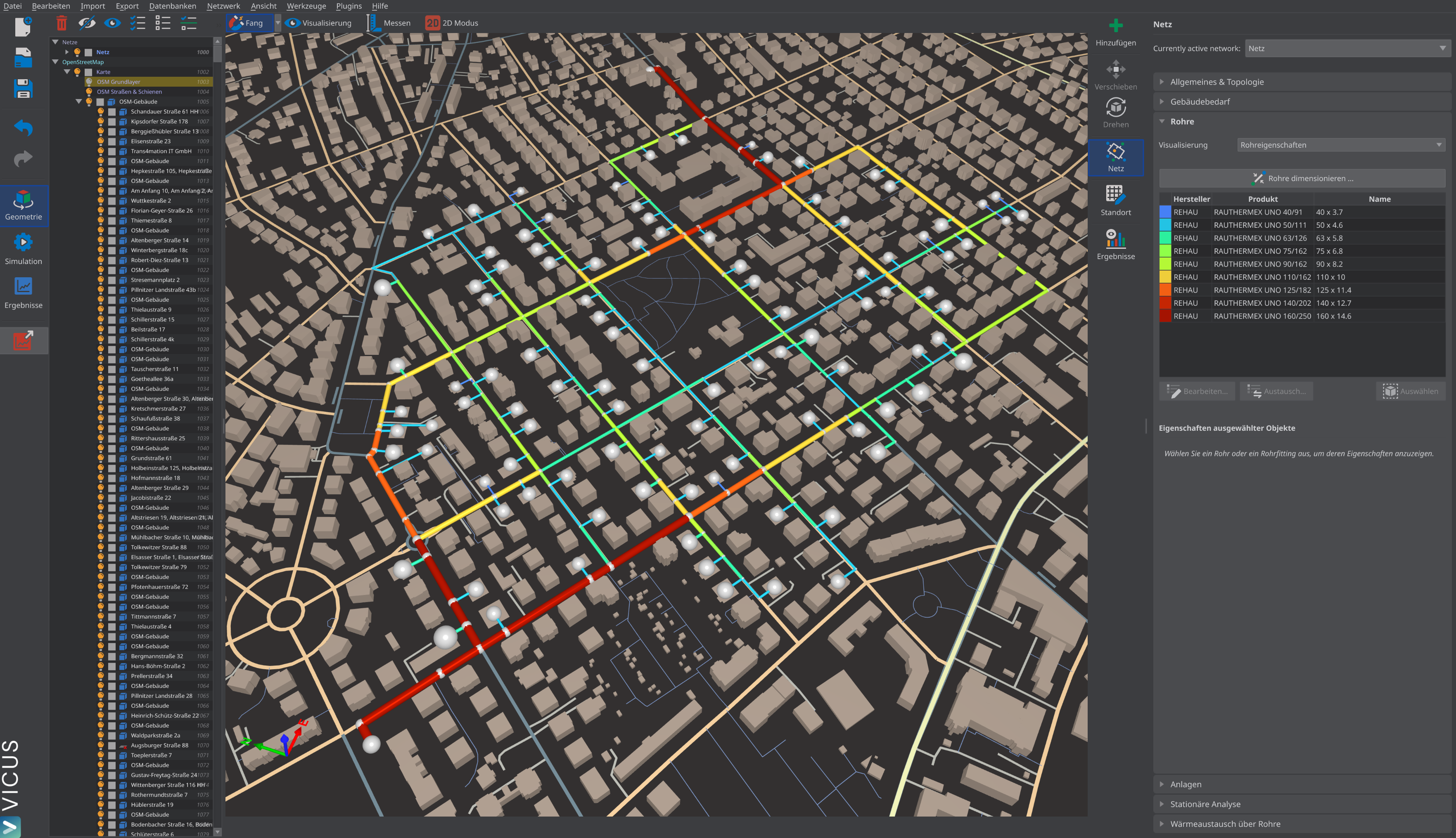
Hydraulic balancing is not a one-time commissioning step. It shapes the efficiency of a district heating network over its whole service life. Static balancing quickly reaches its limits in larger networks with variable load profiles. Automatic differential pressure controllers, combination valves and electronic pressure-independent valves hold the supply quality even at part load and enable energy-efficient pump control. Thermo-hydraulic simulation with tools such as VICUS Districts lets planners quantify the effect of each balancing system on volume flow distribution, return temperatures and pump power consumption already during the planning phase.

Further reading: Transfer Stations describes the design of heat transfer stations where hydraulic balancing is applied, Return Temperature Optimisation shows how correct balancing reduces return temperatures and improves network efficiency, and Pressure Loss Calculation explains the fundamentals of pressure loss determination required for balancing calculations.

References and Standards

• VDI 2073 Part 1 — Hydraulics of water-based systems — Fundamentals
• DIN EN 14336 — Heating systems in buildings — Installation and commissioning of water-based heating systems
• VDI 2035 Part 1 — Prevention of damage in water heating systems — Scale formation and waterside corrosion